Building a suspension kinematics tool | Part III
Multi-link layouts, virtual steering axes, and rifling through the robotics theory parts bin.
Contents:
Introduction
This post is the third in a series on building a tool to simulate the kinematics of a racing car’s suspension. The first post covered the constraint solver itself, and the second covered modelling outboard camber shims, some Jacobian wrangling, and the first batch of metrics.
Since that was posted, the project has had to have a bit of a rebrand. There was already a robotics project using the
name open-kinematics (OpenKinematics), so our suspension tool is now called
Suspension Explorer!
The old open-kinematics solver lives on as the open-core
suspension-explorer-core package, and there’s now a
relatively user-friendly web app sitting in front of it at suspension-explorer.com.
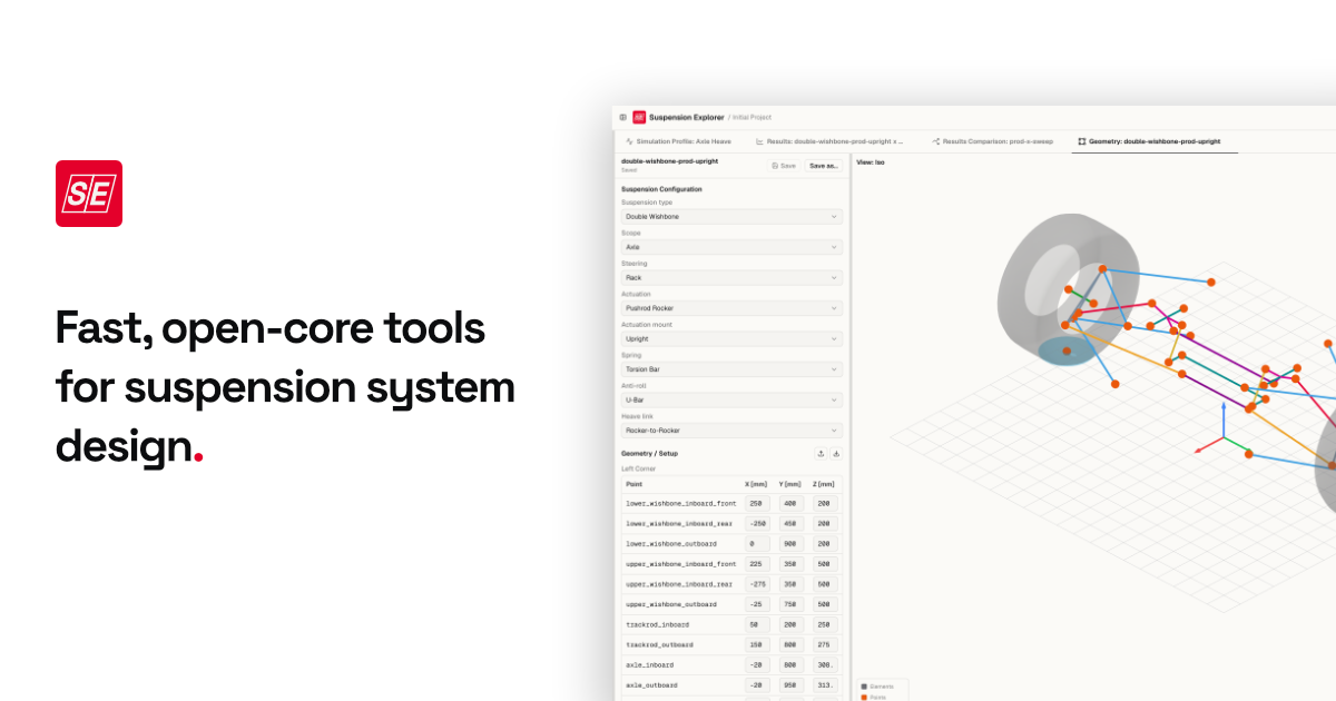
The solver has also picked up some additional functionality: MacPherson struts, trailing arms, a better approach to the road plane, and a good few extra metrics. Most of that was fairly mechanical work on top of the machinery from the first two posts.
However, we also added support for steered multi-link suspensions. Until that functionality was added, the steerable architectures we supported had a physical steering axis: a line through two bearings that the upright would rotate about. This is something multi-link suspension arrangements just don’t have, so we need to do some lifting to work out what the upright actually steers about. To achieve that, we’ve wound up borrowing some screw theory from the world of robotics and bolted it into the analytical derivative machinery described in Part II.
Versions
Multi-link support and the steering response machinery discussed here were first released in
v0.6.1, and the figures and numerical
results in this post were generated with
v0.10.0.
Multi-link
What we mean by multi-link
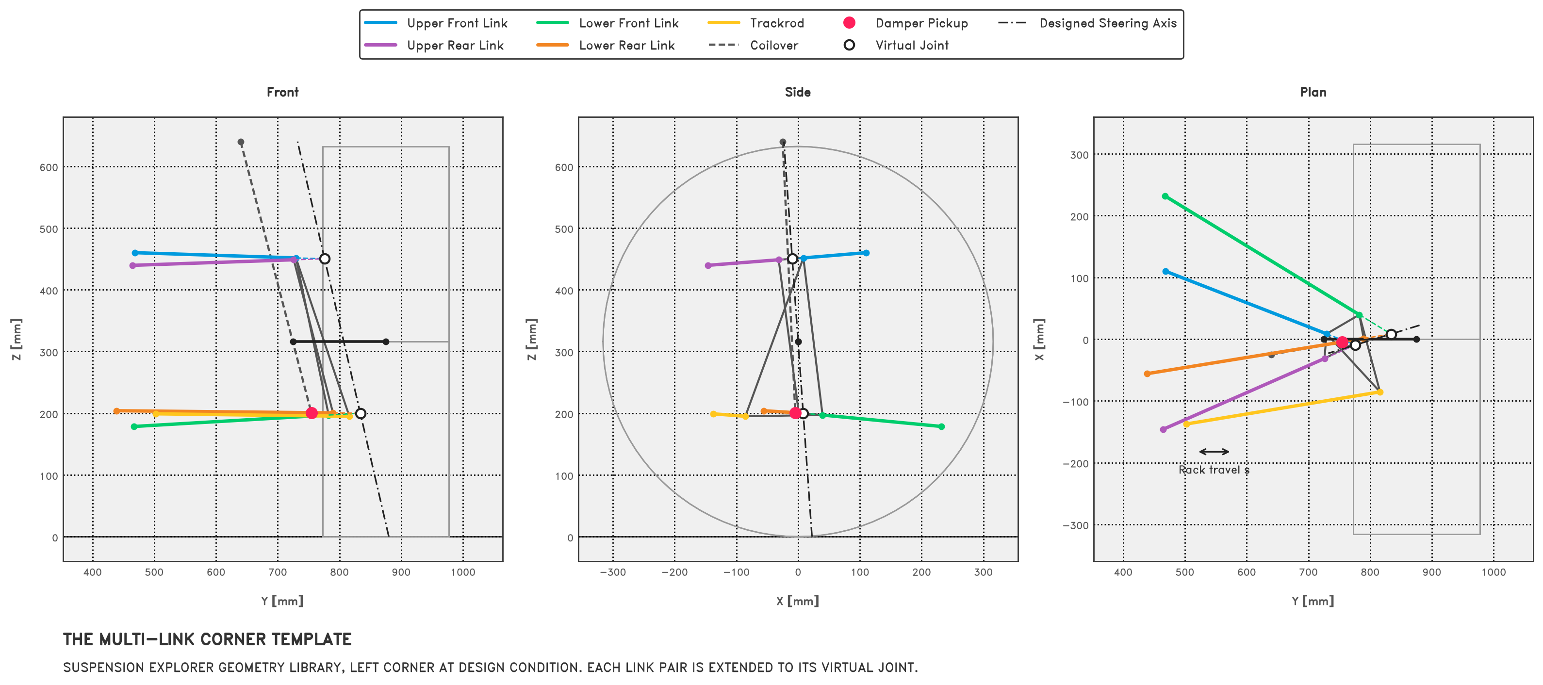
Here, we’re using ‘multi-link’ to mean a five-link setup: four independent locating links, plus a trackrod or toe link. Each link has its own outboard balljoint on the upright, so there are five joints in total. Unlike a double wishbone, there’s no single pair that defines a physical steering axis.
The geometry below is the multi-link corner template from the Suspension Explorer geometry library, and it’s the test geometry used for the rest of this post. It was laid out around a designed steering axis: extend the two upper links until their lines meet, do the same for the two lower links, and at design condition both of those ‘virtual joints’ sit on that axis. We’ll come back to that construction shortly.
On steering axes
Prior to the addition of multi-link support, every steering metric (caster, KPI, scrub radius, mechanical trail etc.) was computed directly from a single steering axis that was defined by the two physical bearings that control how the upright rotates. For example, with a double wishbone setup, it’s simply a line struck through the upper and lower outboard balljoints, $p_{ubj}$ and $p_{lbj}$. A couple of those metric names have changed since Part II; we’ll cover that below.
The multi-link upright still rotates about some sort of axis when the rack moves. If you were to hold the car still, fix the suspension in place†, and cycle the rack… the upright would be rotating about some instantaneous axis, and to compute the steering-axis metrics, we need to find some way to establish what that axis is.
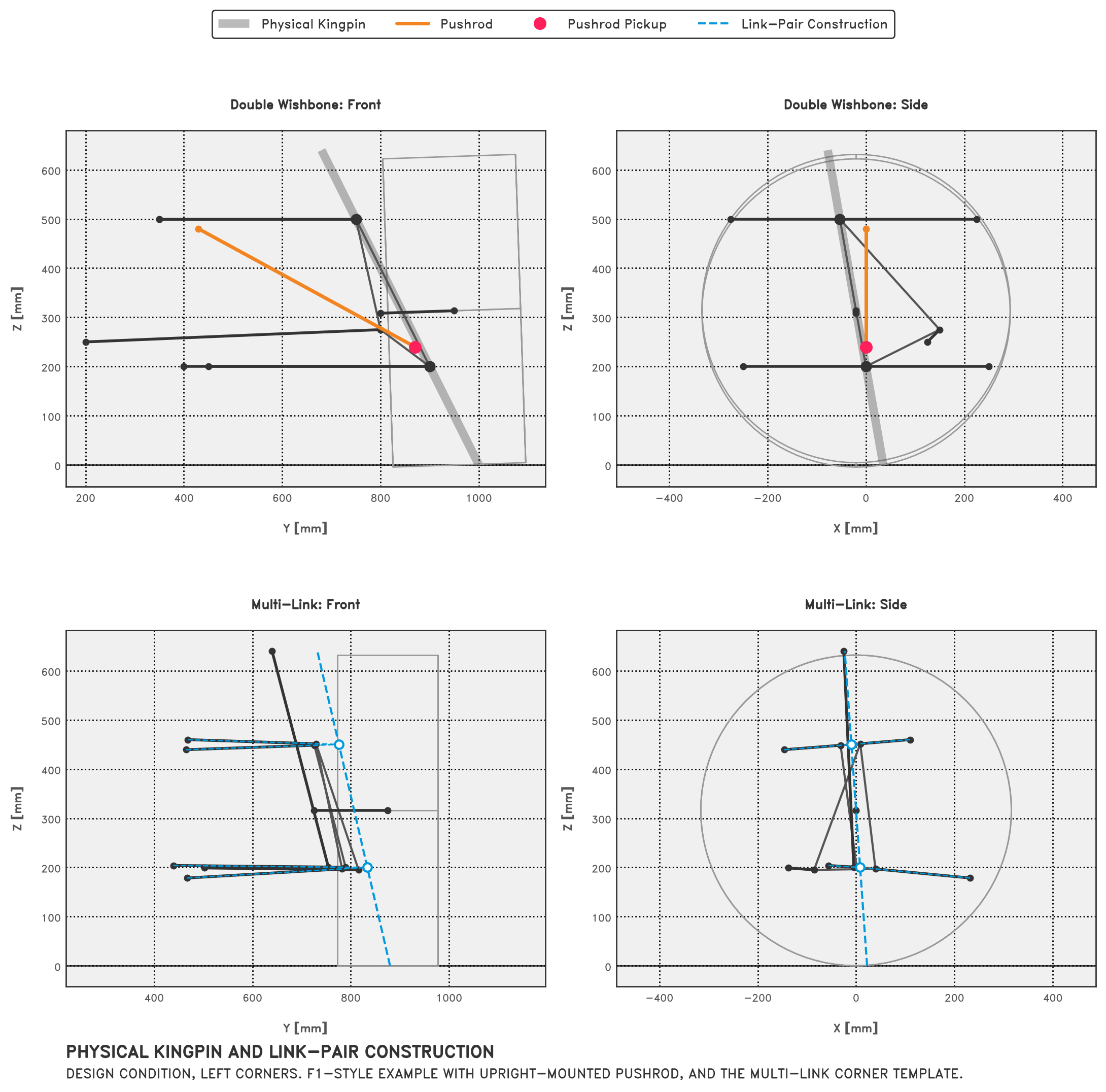
The figure below gives a coarse visualisation of what I mean here. The top plots show that the DWB arrangement has an obvious steering axis defined by two points. This one is the left corner of the F1 style example from the app, with its pushrod moved from the lower wishbone onto the upright, which will matter later. The bottom plots show a multi-link setup, where no single pair of joints defines the axis. In this instance, we can extend the links out to two imagined intersection points, and join those to construct a candidate axis. Whether the upright actually moves about it also depends on what else we hold fixed.
†What exactly we mean by fixed suspension gets kind of complicated here, particularly if your setup couples steering and suspension motion to any substantial degree, but we’ll come to this later.
Extended links and intersection points
As shown in the plot above, one way to construct a candidate axis is to treat each pair of links as a partial or virtual wishbone. Take the two upper links, find where their lines intersect, and call that the virtual upper balljoint, then repeat for the lower pair. The link-pair construction is then just the line connecting your two virtual balljoints.
However, there’s no guarantee the lines will intersect. You could have completely kinematically consistent link arrangements where the link-pair lines never actually intersect. While you could adopt a workaround here, striking the lines to infinity and treating the virtual balljoint position as the midpoint of the closest-approach segment between the two lines, the resulting axis is basically not going to actually describe the motion allowed by the system’s constraints.
So for this tool, I’d like to be able to follow whatever motion the actual constraints allow. Our solver can already compute the positions of everything we care about, including under steer, so the next step is to turn that information into an axis we can use to compute our metrics.
Finding what we’re steering about
The actual implementation of this is fairly gnarly in places, but the general approach is quite straightforward. First, we configure a suspension sweep like any other: set some target displacements or positions for the suspension, e.g., a target wheel centre height or rack bar travel. Then, at each step in the sweep, we:
- Solve for all our point positions as normal.
- Choose which suspension coordinates to hold fixed while the rack moves.
- Compute the response of the upright to an infinitesimal rack displacement, with those coordinates held.
- Fit a rigid-body twist to that response.
- Extract the twist’s screw axis, which is the instantaneous steering axis.
- Hand that axis to the existing caster, KPI, scrub radius, and mechanical trail code.
For Mermaid diagram fans:
flowchart TD
    subgraph sweep["For each step."]
        s1["1: Solve suspension position."] --> s2["2: Choose which suspension coordinates to 'hold' fixed."]
        s2 --> s3["3: Establish upright displacement/response to unit rack displacement."]
        s3 --> s4["4: Fit a rigid-body twist to the upright."]
        s4 --> s5["5: Extract its screw axis/instantaneous steer axis."]
        s5 --> s6["6: Compute caster, KPI, scrub, trail etc."]
        s6 -- "Next step." --> s1
    end
    sweep --> out["Metric curves and the axis surface through travel."]
Some relevant terms here:
- Rigid-body motion: The movement of a body where all points maintain their relative positions.
- Twist: A combined description of a rigid body’s instantaneous translation and rotation.
- Screw axis: The instantaneous axis about which a rigid body rotates, including its direction, a point on it, and the pitch of the motion.
- Screw pitch: The translation along the screw axis per radian of rotation.
The sweep determines the configuration at which we evaluate the suspension. At that configuration, we calculate a separate steering response by moving the rack while holding a chosen suspension coordinate constant. The defaults to hold fixed here are lower wishbone angle for the double wishbone and installed damper length for the multi-link. Damper length here means the installed length of the damper unit, which may or may refer to a coilover setup. In the case of multi-link and the double wishbone coilover template used later, that’s that is a coilovre length; on the F1 style example, which is sprung through torsion bars, it’s the length of the separate damper.
Note that the held values are measured at the current solved state, not at design condition. So the solved sweep tells us where the suspension is, then we hold the suspension there and compute how it would respond to steer input.
flowchart LR
    subgraph sweep["Sweep"]
        targets["Authored<br/>targets."] --> state["Solved<br/>state."]
    end
    subgraph response["Hold and compute"]
        held["Hold at<br/>this state."] --> tangent["Derivative with respect<br/>to rack displacement."] --> axis["Axis and<br/>metrics."]
    end
state --> heldSemantics and reference conditions
At the start, when we said ‘fix the suspension and cycle the rack’, there was a bit more going on than is immediately obvious, at least to me. With a double wishbone setup, you can imagine fixing the wishbones in space and letting the upright rotate about the two outboard balljoints.
However, when we do this, other parts of the system are still moving. With an inclined steering axis and a wheel centre offset from it, steering can move the wheel centre vertically even though neither wishbone moves. If we hold wheel centre height instead, the wishbones have to displace to cancel that vertical motion.
The pushrod arrangement gives us another version of the same problem. With a pushrod mounted on a wishbone, holding the wishbones still also holds the pushrod pickup still. Move that pickup onto the upright, away from the kingpin axis, and steering can drive the pushrod even with the wishbones held. If I hold the inboard rocker still instead, the wishbones may have to move to accommodate the steering. Holding the wishbones and holding the inboard suspension now describe different motions.
For an open-wheel car, ‘fixed internals’ can be a useful way to describe the second experiment: hold the inboard suspension actuation at its current position and move the rack. That still allows motion at the wheel and, with an upright-mounted pushrod, at the wishbones. It doesn’t remove the coupling; that coupling is part of the response.
With multi-link, the locating links themselves may have to articulate for the upright to steer; there isn’t a pair of wishbones we can freeze to isolate the kingpin axis. We therefore need to say what we’re holding fixed when we describe its steering response. Otherwise, a comparison between two layouts can also contain a difference in how we’ve constrained them.
We’ll compare the different holds once we can see what the fitted axis does. For a double wishbone with a wishbone angle held, the whole process should give us back the physical steer axis, which gives us a useful check that it’s all working as intended.
Building the multi-link model
Building the linkage itself is fairly straightforward. We can reuse the constraints from the earlier posts:
- Four distance constraints, one per link, each preserving its balljoint-to-balljoint length.
- A rigid upright: the first three points form a base triangle (three mutual distances), and every other upright point is anchored to that triangle, preserving which side of it the point started on so the solver can’t flip the upright into a mirrored arrangement.
- An explicit axle length constraint between the two axle points, so the wheel axis can’t drift inside the redundant upright constraint set.
- The trackrod or toe link, actuation, spring, and damper constraints, composed through the same mechanism fields as the double wishbone.
For the damper, the only option we currently have is to mount it on the centreline of the lower link at some distance along it. This is not very representative of an F1 style multi-link layout, but does broadly match the multi-link road car layouts I’ve laid eyes upon… and we can always expand this.
As an aside for the more software-minded people, making the physical steering axis optional also had some knock-on effects in the codebase. Any architecture can now report that it has no physical steering axis, in which case the physical caster, KPI, etc. columns are dropped from the output, and only the virtual family appears.
Rack displacement response
Step 3 of the Mermaid diagram is to work out how every point on the upright responds to a change in rack displacement at a given solved state.
If we call the rack displacement $s$, then for each point $p_i$ we want to establish the derivative of its position with respect to rack displacement:
$$ r_i = \frac{\partial p_i}{\partial s} $$Each $r_i$ has three components, one for each chassis direction ($x, y, z$), measured in millimetres of point displacement per millimetre of rack displacement. This is the point’s rate of change of position with respect to rack travel.
For example, a vertical component of $+0.2$ mm/mm means a $+0.1$ mm rack displacement would induce $+0.02$ mm of vertical point displacement. This derivative describes the response at the current configuration only, with the chosen suspension coordinate held, and it can also change as the linkage moves.
In code and elsewhere we refer to these derivatives wrt. rack displacement simply as ‘rates’; the variable naming
convention uses _rate suffixes as a shorthand for rate of change with respect to rack travel.
A note on notation: in Part I and Part
II, $r$ was reserved for solver residuals, with $r_i$ the
$i$-th residual component in the Jacobian definition. In this post, $r_i$ is instead the rate of point $i$ with respect
to rack displacement. That matches the rates, reference_point_rate, and rotation_rate_vector names in the code,
which is where this derivation lives. Residuals do still appear below, but only as norms like $\|A x - b\|$, so the two
meanings don’t collide within this post.
Still no finite differences
The obvious way to get these derivatives is to perturb the rack by some small $\delta$, keeping the same suspension coordinates held. Then, we’d re-solve for all our positions and divide the change in relevant point position coordinates by $\delta$.
That would work, but having gone to some lengths to get analytical derivatives already (see Part II), I’d quite like us to use them here as well.
Reusing our Jacobian
Thankfully, Part II already did most of the work. We have the analytical Jacobian, so we can fish out how the points would move for an infinitesimal rack travel input without actually having to perturb the rack and re-solve the suspension state. We’re still limited by floating-point arithmetic and the accuracy of the solved configuration, but we’re already in a good spot, so:
Let $q$ be the vector of free point coordinates; Part II wrote this vector as $x$, and $q$ is what the solver code calls it. At a given solved state, the permanent mechanism constraints are satisfied:
$$ C(q) = 0 $$These are the link lengths, the upright rigidity, the rack guide etc. For the steering response, we choose a set of scalar coordinates $g(q) = t$: rack displacement and the selected suspension holds, with their values taken from the current solved state. This uses the same machinery as a sweep’s targets, but the choice of coordinates is separate. Differentiating the full residual $[C(q),\; g(q) - t] = 0$ with respect to target $t_j$ gives:
$$ \begin{bmatrix} C_q \\ g_q \end{bmatrix} \frac{\partial q}{\partial t_j} = \begin{bmatrix} 0 \\ e_j \end{bmatrix} $$Where $C_q$ and $g_q$ are the constraint and target Jacobians, and $e_j$ is the $j$-th unit vector. That is, we want a direction of motion that keeps every constraint satisfied, gives target $j$ a derivative of one, and gives every other target a derivative of zero, all with respect to $t_j$. This is a single linear solve at the current configuration, with no perturbation and no extra nonlinear solve.
When target $j$ is the rack displacement, $\partial q / \partial t_j$ is the derivative with respect to $s$ that we’re after, and each $r_i$ contains its three components for point $i$. The other targets in the basis are the coordinates held fixed in that derivative.
Solving in the null space
We could throw that stacked system straight into another least-squares solve, but there’s a useful way to break up the task here, which I picked up in my day job while working on a CAD system sketch solver. First, we need to work out which motions the links and joints permit. Then we can work out which combination of those motions satisfies our targets. This also lets us see whether we’ve supplied enough targets to choose a unique answer.
First, any valid direction of motion $\delta q$ must keep the permanent constraints satisfied, i.e., $C_q\, \delta q = 0$, so it must lie in the null space of $C_q$. We get an orthonormal basis $N$ for that null space from a singular value decomposition (SVD):
$$ C_q = U \Sigma V^\top, \qquad N = V_{[:,\, k:]} $$Where $k$ is the numerical rank of $C_q$ and $n$ is the number of free coordinates. The number of columns of $N$, $m = n - k$, is the mechanism’s local ‘mobility’, i.e., the number of independent ways it can move at this configuration. For a steered corner, $m$ is typically two; one for suspension travel, and one for the rack.
Every valid/permissible motion is then $\delta q = N \alpha$ for some $\alpha \in \mathbb{R}^m$, and the target equations shrink to a small $n_{targets} \times m$ system:
$$ (g_q N)\, \alpha_j = e_j, \qquad \frac{\partial q}{\partial t_j} = N \alpha_j $$In sensitivity.py, $N$ is the trailing block of right singular vectors from the SVD of the row-normalised constraint Jacobian:
_left, singular_values, right_transpose = np.linalg.svd(
    normalized,
    full_matrices=True,
)
rank = _singular_value_rank(singular_values, normalized.shape)
return _ConstraintTangentSpace(
    basis=right_transpose[rank:].T.copy(),
    rank=rank,
    singular_values=tuple(float(value) for value in singular_values),
)
and the reduced solve in
compute_state_tangents
is the small system above, with constraint_space.basis as $N$ and the identity as the stacked right-hand sides $e_j$:
restricted_targets = target_jacobian @ constraint_space.basis
normalised_targets, row_scales = _normalise_rows(restricted_targets)
target_right_hand_sides = np.eye(n_targets, dtype=np.float64)
normalised_right_hand_sides = row_scales[:, None] * target_right_hand_sides
reduced_tangents, target_rank, target_singular_values = _solve_reduced_responses(
    normalised_targets,
    normalised_right_hand_sides,
    constraint_space.mobility,
    n_targets,
)
tangent_arrays = constraint_space.basis @ reduced_tangents
combined_rank = constraint_space.rank + target_rank
full_column_rank = combined_rank == computer.n_vars
Splitting things up this way has a few advantages:
- The constraint derivatives are zero by construction, so the target rows can’t trade off against constraint satisfaction as they might in a single stacked least-squares solve.
- The mobility can be reported. If the targets don’t span the mechanism’s motion, i.e., $\text{rank}(g_q N) < m$, the response isn’t unique, and the solver reports it as such; it won’t silently fall back to the minimum-norm solution.
- A one-DOF mechanism that needs no extra holds is handled without any special case fiddling.
- How well each target couples to the mechanism can be measured with a projection ratio. For row $i$ of $g_q$, this is $\|g_{q,i}\, N\| / \|g_{q,i}\|$. A ratio near zero means target $i$ is nearly orthogonal to every motion the mechanism can make, so a small change in that target would require a large change in the free point coordinates.
After the solve, the residuals of the differentiated constraint and target equations are checked again with scale-aware tolerances. Redundant holds that are consistent with the requested rack response will pass, while conflicting ones will be flagged.
Propagating to derived points
The null space solve gives derivatives for the free points only, but derived points, such as the wheel centre and contact patch, need them too. Part II already built the right tool for this in the dual number type. So, we seed each free point’s dual number with its position and its derivative with respect to rack displacement, run the derived point dependency graph, and read off the resulting derivatives.
At this point, every point on the upright has a position $p_i$ and a derivative with respect to rack displacement, or rate, $r_i$. That combination is all we need to fit a rigid-body motion and extract the screw axis.
At each solved state, the fit runs once, with the tangent field from the hold and the upright’s own point keys; see compute_steering_response_axes in steering_axis.py.
Rigid-body motion, twist, and screw axis theory
Rigid-body motion
We should now have both position and rate information for every point, so what we want next is a description of the upright’s motion as a unit. By treating the upright as a rigid body, we assume that the distances between its attached points stay constant.
By doing this, we don’t have to describe every point’s motion independently. If we know how the body is rotating and translating, we know what all of the attached points are doing. For reference, Modern Robotics (pp. 12–15) gives a useful introduction to rigid bodies and their degrees of freedom.
As a side note, in the dynamics/robotics world where we’ve gone digging for techniques to steal, motion is usually described as a function of time. However, the Lynch and Park book does separate a scalar path parameter from time on pp. 325–326, and our $s$ plays exactly that role. They also call it $s$, though theirs is normalised to $[0, 1]$ where ours is absolute rack displacement.
In terms of the actual rigid-body stuff, any rigid motion can be written as a rotation plus a translation; this is the point transformation on p. 90. If $b_i$ is the constant position of point $i$ in a frame attached to the upright, then its position in the chassis frame is:
$$ p_i(s) = R(s)\, b_i + \tau(s) $$Where $R$ is the rotation matrix taking body space directions into the chassis frame, and $\tau$ is the position of the body space origin in chassis coordinates, i.e., the translation. With the chosen hold fixing our path through the configurations, we’ll write derivatives along that path with a prime, $r_i = p_i' = dp_i/ds$:
$$ r_i = R' b_i + \tau' = R' R^\top (p_i - \tau) + \tau' $$Since $R R^\top = I_3$, differentiating gives $R' R^\top + R R'^\top = 0$, which tells us that $R' R^\top$ is skew-symmetric: its transpose is its negative. Every $3 \times 3$ skew-symmetric matrix can represent a cross product with a vector. This is the skew-symmetric representation of a rotation derivative used on pp. 77–78, with differentiation now taken with respect to $s$:
$$ R' R^\top = [\rho]_\times = \begin{bmatrix} 0 & -\rho_z & \rho_y \\ \rho_z & 0 & -\rho_x \\ -\rho_y & \rho_x & 0 \end{bmatrix}, \qquad [\rho]_\times v = \rho \times v $$So, if we pick any reference point $p_{ref}$ on the body, with derivative $r_{ref}$ with respect to rack displacement, the derivative of every other point on the body follows:
$$ r_i = r_{ref} + \rho \times (p_i - p_{ref}) $$Here, $\rho$ is the upright’s angular rate with respect to rack travel, in radians per millimetre. For a small rack increment $\Delta s$, $\rho\,\Delta s$ describes the corresponding small rotation in the chassis frame.
However many points the upright carries, then, the instantaneous motion of all of them is described by six numbers: three for $r_{ref}$ and three for $\rho$. In robotics, this combined description is called a ’twist’; see p. 99.
Here, we take the linear part at $p_{ref}$ and express both vectors along the chassis axes. The book’s spatial twist uses the fixed frame origin instead; its corresponding linear part would be $r_{ref} - \rho \times p_{ref}$ in our notation, with both parts still measured per millimetre of rack.
Fitting the twist
The rigid-body relation describes the upright’s response with six numbers, $(r_{ref}, \rho)$. What we actually have is a set of positions $p_i$ and derivatives $r_i$ for the points on the upright, so we need to get from the points to the twist.
Rearranging that relation using $\rho \times d = -d \times \rho = -[d]_\times \rho$, with $d_i = p_i - p_{ref}$:
$$ r_i = r_{ref} - [d_i]_\times\, \rho = \begin{bmatrix} I_3 & -[d_i]_\times \end{bmatrix} \begin{bmatrix} r_{ref} \\ \rho \end{bmatrix} $$Each point gives us three equations in six unknowns, so stacking all $n_p$ points on the upright gives a $3n_p \times 6$ linear system, $A x = b$, with $x$ the stacked unknown $(r_{ref}, \rho)$:
$$ \underbrace{ \begin{bmatrix} I_3 & -[d_1]_\times \\ I_3 & -[d_2]_\times \\ \vdots & \vdots \\ I_3 & -[d_{n_p}]_\times \end{bmatrix} }_{A} \underbrace{ \begin{bmatrix} r_{ref} \\ \rho \end{bmatrix} }_{x} = \underbrace{ \begin{bmatrix} r_1 \\ r_2 \\ \vdots \\ r_{n_p} \end{bmatrix} }_{b} $$The fit uses the points the UprightElement declares: the four link balljoints, the two axle points, and the trackrod
outboard joint; seven in total on the test geometry. A damper pickup that ties into a link is a derived point on that
link, not an upright point, so it isn’t included. Seven points give 21 equations in six unknowns, so the system is
overdetermined, and we can solve it with least squares. Here’s the fitting section from
fit_rigid_body_twist in screw_axis.py
at v0.10.0:
point_positions = selected.positions
point_rates = selected.rates
reference = np.mean(point_positions, axis=0)
offsets = point_positions - reference
geometry_scale = float(np.sqrt(np.mean(np.sum(offsets**2, axis=1))))
rate_scale = float(np.sqrt(np.mean(np.sum(point_rates**2, axis=1))))

design = np.empty(
    (3 * len(selected.keys), _RIGID_BODY_TWIST_DOF),
    dtype=np.float64,
)
for index, offset in enumerate(offsets):
    rows = slice(3 * index, 3 * index + 3)
    design[rows, :3] = np.eye(3)
    design[rows, 3:] = -_skew_symmetric(offset)

solution, _residuals, rank, _singular_values = np.linalg.lstsq(
    design,
    point_rates.reshape(-1),
    rcond=None,
)
fitted_rates = (design @ solution).reshape(-1, 3)
residual_norms = np.linalg.norm(fitted_rates - point_rates, axis=1)
fit_rms = float(np.sqrt(np.mean(residual_norms**2)))
fit_max = float(np.max(residual_norms))
Here, _RIGID_BODY_TWIST_DOF is six. The first three entries of solution give the reference point’s rate with respect
to rack travel, and the last three give the rotation rate vector.
The code uses the centroid of the fitted points as $p_{ref}$, which separates the translational and rotational parts of the least-squares fit; there’s a short derivation of why in the aside at the end.
Screw axis theory
While the ’twist’ concept describes the motion, it doesn’t directly give us the axis the upright is steering about. For that, we can lean on a result credited to Mozzi and Chasles:
Any instantaneous rigid-body motion with nonzero rotation is a rotation about a unique line plus a translation along that same line.
That line is the ‘instantaneous screw axis’ (ISA), and like the screw axes you’ll be familiar with, the ratio of translation to rotation is its ‘pitch’, $h$.
Locating the axis takes little work. We want a point $c$ whose position derivative with respect to rack displacement is parallel to $\rho$, since points on the screw axis only slide along it:
$$ r_c = r_{ref} + \rho \times (c - p_{ref}) \parallel \rho $$Try $c - p_{ref} = \dfrac{\rho \times r_{ref}}{|\rho|^2}$. Using the vector triple product $\rho \times (\rho \times r) = \rho (\rho \cdot r) - r (\rho \cdot \rho)$:
$$ \begin{aligned} r_c &= r_{ref} + \frac{\rho \times (\rho \times r_{ref})}{|\rho|^2} \\ &= r_{ref} + \frac{\rho (\rho \cdot r_{ref})}{|\rho|^2} - r_{ref} \\ &= \frac{\rho \cdot r_{ref}}{|\rho|^2}\, \rho \end{aligned} $$That’s parallel to $\rho$, as required, so the screw axis is the line:
$$ c = p_{ref} + \frac{\rho \times r_{ref}}{|\rho|^2}, \qquad \hat{a} = \frac{\rho}{|\rho|} $$Then the pitch, i.e., the translation along the axis per radian of rotation, is:
$$ h = \frac{\rho \cdot r_{ref}}{|\rho|^2} $$The point $c$ is also the point on the axis closest to $p_{ref}$, since $c - p_{ref}$ is perpendicular to $\rho$ by construction.
That whole derivation is the tail of
extract_screw_axis in screw_axis.py,
with rotation_rate_vector as $\rho$, angular_rate as $|\rho|$, and reference_point_rate as $r_{ref}$:
angular_rate_squared = angular_rate**2
direction = rotation_rate_vector / angular_rate
closest_point = twist.reference_point.data + (
    np.cross(rotation_rate_vector, reference_point_rate) / angular_rate_squared
)
pitch = float(
    np.dot(rotation_rate_vector, reference_point_rate) / angular_rate_squared
)
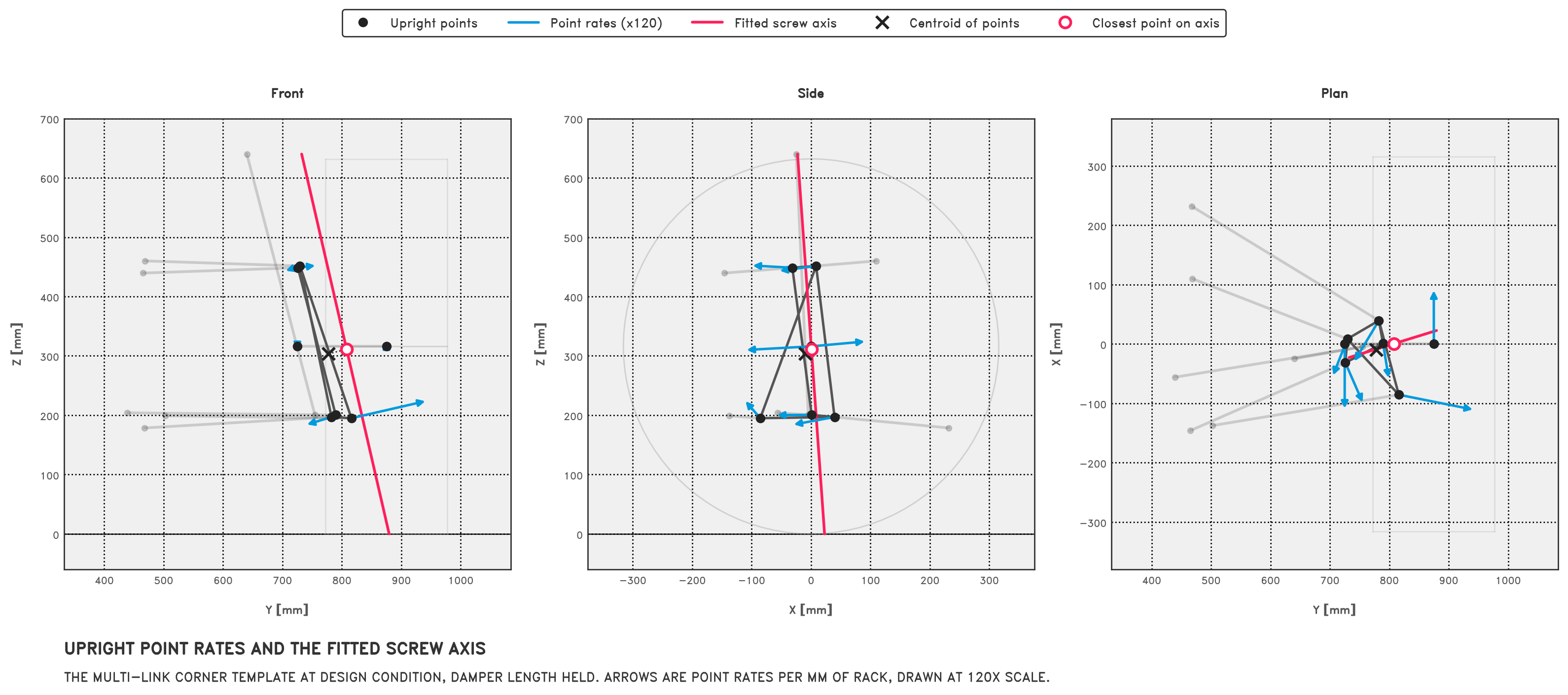
Putting the fit and the extraction together for the multi-link template at design condition, the inputs and the output look like this. The arrows are the point rates $r_i$ that fill $b$, and the red line is the axis recovered from the fitted $x$. In the plan view the arrows circulate about the axis, and points further from it move faster, as they should for a rotation. The cross is the centroid of the points, which the code uses as $p_{ref}$, and the hollow marker is $c$, the point on the axis closest to it.
A few properties of this will come up again later:
- The axis doesn’t depend on the scale of the derivatives. Doubling every $r_i$ doubles $\rho$ and $r_{ref}$ together, which leaves $c$, $\hat{a}$, and $h$ unchanged; only the angular rate with respect to rack travel, $|\rho|$, changes. So it doesn’t matter whether we measure per millimetre of rack or per metre.
- The axis doesn’t depend on the choice of $p_{ref}$. Moving the reference point changes $r_{ref}$ by exactly the amount needed to give back the same axis.
- The direction has no meaningful sign. Reversing the rack reverses $\rho$, but the axis is the same. When comparing axes, we use $|\hat{a}_1 \cdot \hat{a}_2|$, and when computing metrics, we flip the direction to point chassis-up so that caster and KPI come out with the usual signs.
- For a double wishbone with a wishbone angle held, the pitch should be zero. Both balljoints are stationary to first order in a regular configuration, so the upright purely rotates about the line through them. This makes for a useful check later on.
None of this is new. It’s the foundation of Ball’s Theory of Screws (1876), and Lynch and Park cover it on pp. 99–103, where twists and screw axes are the standard way to describe the motion of a robot’s links.
When the fit goes wrong
We also need to know when the fit or axis extraction isn’t giving us anything useful. The code returns a
ScrewAxisStatus for each frame: VALID or one of six failure statuses, so a bad frame is recorded and the rest of the
sweep carries on. Four of the failure statuses cover the following geometry and motion checks:
- Too few or degenerate points: fewer than three usable points (
INSUFFICIENT_POINTS), or points that are coincident or collinear (DEGENERATE_GEOMETRY). The second is checked with an SVD of the centred positions; if the second singular value is tiny relative to the first, the points span at most a line. - Excessive fit error (
EXCESSIVE_FIT_ERROR): if the derivatives really came from a rigid body, every point’s residual $r_i - (r_{ref} - [d_i]_\times \rho)$ should be zero to numerical precision. The code checks the largest per-point residual norm,fit_max, against $10^{-5}$ times the RMS point rate, with an absolute floor of $10^{-10}$. A large residual means something upstream is broken, e.g., a point has been wrongly assigned to the upright, or a constraint isn’t holding it rigid. The fit residual therefore doubles as a rigidity check on the point derivatives. - Near-pure translation (
NEAR_PURE_TRANSLATION): if rotation is negligible relative to the point motion, the axis can become arbitrarily distant or poorly determined. From the extraction formula, its distance from the reference point is $|c - p_{ref}| = |r_{ref,\perp}| / |\rho|$, where $r_{ref,\perp}$ is the component of the reference point rate perpendicular to $\rho$. A translation parallel to $\rho$ increases the pitch without moving the axis sideways. As rotation vanishes, a pure translation has no unique finite axis location, though it can be represented by a screw of infinite pitch along the translation direction. Without this check, a small rounding error in $\rho$ could put the axis somewhere unfeasibly far away.
The other two, RANK_DEFICIENT and NON_FINITE, catch a least-squares matrix of rank below six and any non-finite
value in the inputs or the solution.
flowchart TD
    in["Upright positions and rates."] --> count{{"Three or more usable points."}}
    count -.-> insufficient["Insufficient points."]
    count --> geom{{"Points not collinear."}}
    geom -.-> degenerate["Degenerate geometry."]
    geom --> fit["Least-squares twist fit."]
    fit --> rank{{"Rank six, all values finite."}}
    rank -.-> rankdef["Rank deficient or non-finite."]
    rank --> residual{{"Largest point residual within tolerance."}}
    residual -.-> error["Excessive fit error."]
    residual --> rotation{{"Angular rate above threshold."}}
    rotation -.-> translation["Near-pure translation."]
rotation --> valid["Valid screw axis."]The threshold for that last check needs some care, since $|\rho|$ is in radians per unit $s$, while the point derivatives are in millimetres per unit $s$. Dividing the RMS point derivative by the RMS distance of the points from the centroid gives a characteristic angular rate with respect to rack travel, so the threshold is set relative to that:
$$ |\rho| \le \epsilon \cdot \frac{\text{rms}(r_i)}{\text{rms}(d_i)} \quad \Rightarrow \quad \text{near-pure translation} $$This relative criterion is independent of units, body size, and the scale of the driving parameter. The principal
tolerances are scaled to the geometry and rates, with absolute floors for vanishing values. In the code, $\epsilon$ is
_ANGULAR_RATE_RELATIVE_TOLERANCE, which is $10^{-8}$, and the threshold is built in
extract_screw_axis in screw_axis.py.
Steering metric conventions
Before comparing the axes, a quick update on the metric names. Since Part II, we’ve aligned the ground metric definitions with ISO 8855:2011:
- Ground offset is the signed lateral distance from the tyre contact centre to the steering-axis intersection with the local road plane, measured along the tyre’s lateral direction and positive when the intersection is inboard. This is the quantity I called scrub radius in Part II.
- Scrub radius is the full, unsigned distance between those two points in the road plane.
- Mechanical trail is their fore-aft separation along the steered tyre’s forward direction, positive when the axis intersection is ahead of the contact centre. Part II measured this along chassis X.
So ground offset and mechanical trail are the lateral and longitudinal components of the same displacement, while scrub radius is its magnitude.
The plots also include lateral and longitudinal steering-axis offsets at wheel centre height. For those, we intersect the axis with a plane through the wheel centre, parallel to the local road, and resolve the displacement from the wheel centre along the tyre’s lateral and forward directions. Lateral offset is positive inboard, like ground offset. Longitudinal offset is positive when the axis is behind the wheel centre, which is the opposite sign to mechanical trail, so watch out for that one when reading the plots. Caster ties the two together: with the wheel centre at height $h_{wheelCenter}$ above the road,
$$ t_{mechanical} \approx h_{wheelCenter} \tan(\theta_{caster}) - o_{longitudinal} $$This relationship can be a bit deceptive because of the definitions: caster is measured in the chassis XZ plane, while trail and longitudinal offset are measured along the steered tyre’s forward direction. The approximation is useful near straight ahead, with the road parallel to the chassis XY plane; at larger steer angles those directions differ, so it probably shouldn’t be used to reconstruct trail throughout the sweep.
On the double wishbone coilover template plotted below, $h_{wheelCenter} \tan(\theta_{caster})$ is 26.1 mm at design condition and the longitudinal offset is −10.5 mm. The axis is 10.5 mm ahead of the wheel centre at hub height, and leans back to 36.7 mm ahead of the contact centre at the ground; negative longitudinal offset and positive trail both mean ‘ahead’.
We’ll use these definitions for both the physical and virtual axes in the comparisons below.
Sanity checking our work: recovering a DWB kingpin axis
Conveniently, the double wishbone model means we know what answer to expect.
For a double wishbone, one ’natural’ seeming hold is the lower wishbone’s angle about its inboard hinge axis. With that held, the lower arm is locked, so $p_{lbj}$ is stationary. With $p_{lbj}$ stationary and the upright rigid, $p_{ubj}$ is constrained to the intersection of a circle (the upper arm’s swing) and a sphere (centred on $p_{lbj}$). Away from singular configurations, those constraints make $p_{ubj}$ stationary too. Both balljoints have zero derivatives with respect to rack displacement, and the only motion left is a pure rotation about the line through them, which means the virtual axis is the physical kingpin.
Holding the upper wishbone angle instead gives the same answer, since either arm angle is a valid local coordinate for suspension travel.
So with either wishbone angle held, the fitted axis should go straight through the two balljoints. We can check that while moving the suspension through a fairly varied set of configurations.
The test suite (test_moving_dampers_recover_physical_axis_at_every_state) solves a mirrored double wishbone axle through a combined bump and steer sweep, with damper lengths changing by more than 10 mm, and checks at every frame that:
- The virtual axis direction matches $p_{ubj} - p_{lbj}$ to $|\hat{a}_{virtual} \cdot \hat{a}_{physical}| = 1 \pm 10^{-10}$;
- Both balljoints lie within $10^{-8}$ mm of the fitted axis;
- The pitch is zero to within $10^{-8}$ mm/rad;
- Both balljoint derivatives are zero to within $2 \times 10^{-10}$ mm/mm.
So, we can recover the steer axis to numerical precision at every state in this combined bump and steer test sweep.
The full metric set
With the axis recovered, we can get back to the sort of quantities we’d actually want to plot for a suspension.
Thankfully, Part II already covered most of the work here. We convert the fitted screw axis into the same SteeringAxis
type used for the physical kingpin: a point and a direction, with the direction flipped to point chassis-up
(SteeringAxis.from_unoriented_line in metrics/steering.py):
@classmethod
def from_unoriented_line(
    cls,
    point: Point3,
    direction: Vector3 | Direction3,
) -> SteeringAxis:
    """Construct an axis from a line whose input direction has no meaning.

    The sign is chosen chassis-up when possible, with deterministic X/Y
    tie-breakers for a horizontal line. This suits screw-axis fits, whose
    line direction may be reversed without changing their geometry.
    """
    axis = cls.from_point_direction(point, direction)
    canonical = axis.direction
    for component in (Axis.Z, Axis.X, Axis.Y):
        if abs(canonical[component]) >= EPS_GEOMETRIC:
            if canonical[component] < 0.0:
                canonical = -canonical
            break
    return cls.from_point_direction(axis.point, canonical)
From there, caster, KPI, ground offset, scrub radius, and mechanical trail are computed by the same functions for both
physical and virtual axes, using the conventions above. The metric code has no knowledge
of where the axis came from. The virtual family is reported with a _virtual suffix.
The fit also provides two extra quantities:
- Screw pitch. A nonzero pitch means the motion includes translation along the steering axis. For a double wishbone with either wishbone angle held, it’s zero; for a multi-link, it describes the axial translation in the selected steering response. It depends on the hold as well as the mechanism.
- Angular rate with respect to rack travel. $|\rho|$ measures the upright’s total rotation per millimetre of rack at the current state. Wheel steer is a heading angle in the chassis XY plane, so its derivative is generally different.
The same double wishbone test checks that caster, KPI, ground offset, scrub radius, and mechanical trail computed from the virtual axis match the physical values to within $10^{-8}$ in each metric’s native units (degrees for angles, mm for distances). The figure below runs the same kind of sweep on the F1 style example from earlier, with the rack running ±40 mm while the two dampers move in opposite directions (16 mm of travel on the left):
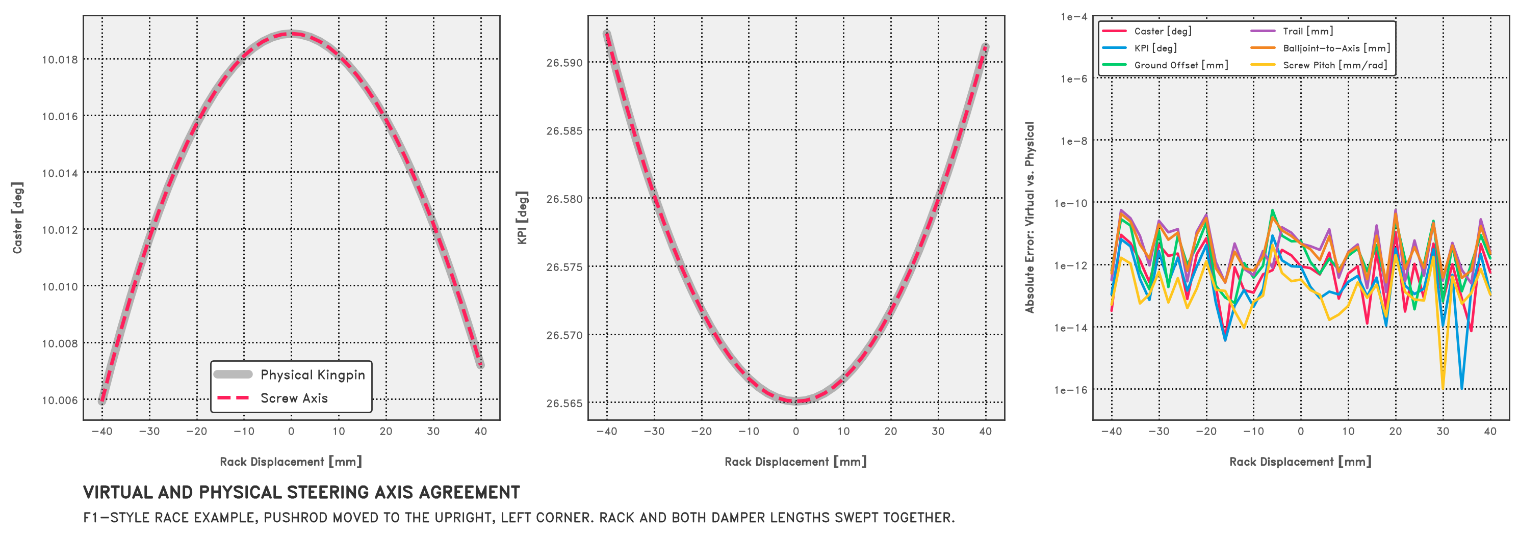
The physical and virtual curves sit on top of one another, so the error plot on the right is more useful than the overlaid traces. In each metric’s native units, the largest error is around $5 \times 10^{-11}$, and most values sit between $10^{-13}$ and a few times $10^{-11}$.
We can also run the same comparison on a second double wishbone, the app’s double wishbone with coilover template, and plot every steering metric rather than just checking deltas. In place of the F1 style example’s pushrod, rocker, and torsion bars, it has a coilover mounted directly on the lower wishbone. It also has a physical kingpin, so each metric can be computed twice: once from the line through the two balljoints, and once from the screw axis fitted to the steering response with the template’s default hold, lower wishbone angle. The plots below overlay the two through ±60 mm of bump and ±40 mm of rack, the same sweeps we’ll use for the multi-link below, with the physical kingpin drawn thick and grey and the screw axis dashed on top.
For both templates, the sweep conditions are:
| Sweep | Varied coordinate | Held coordinate |
|---|---|---|
| Bump | Wheel centre height, ±60 mm from design | Rack displacement |
| Steer | Rack displacement, ±40 mm from design | Wheel centre height |
At every solved state in either sweep, we calculate a separate steering response with the current lower wishbone angle held for the double wishbone, or the current damper length held for the multi-link. Those response holds are independent of the held coordinates in the table.
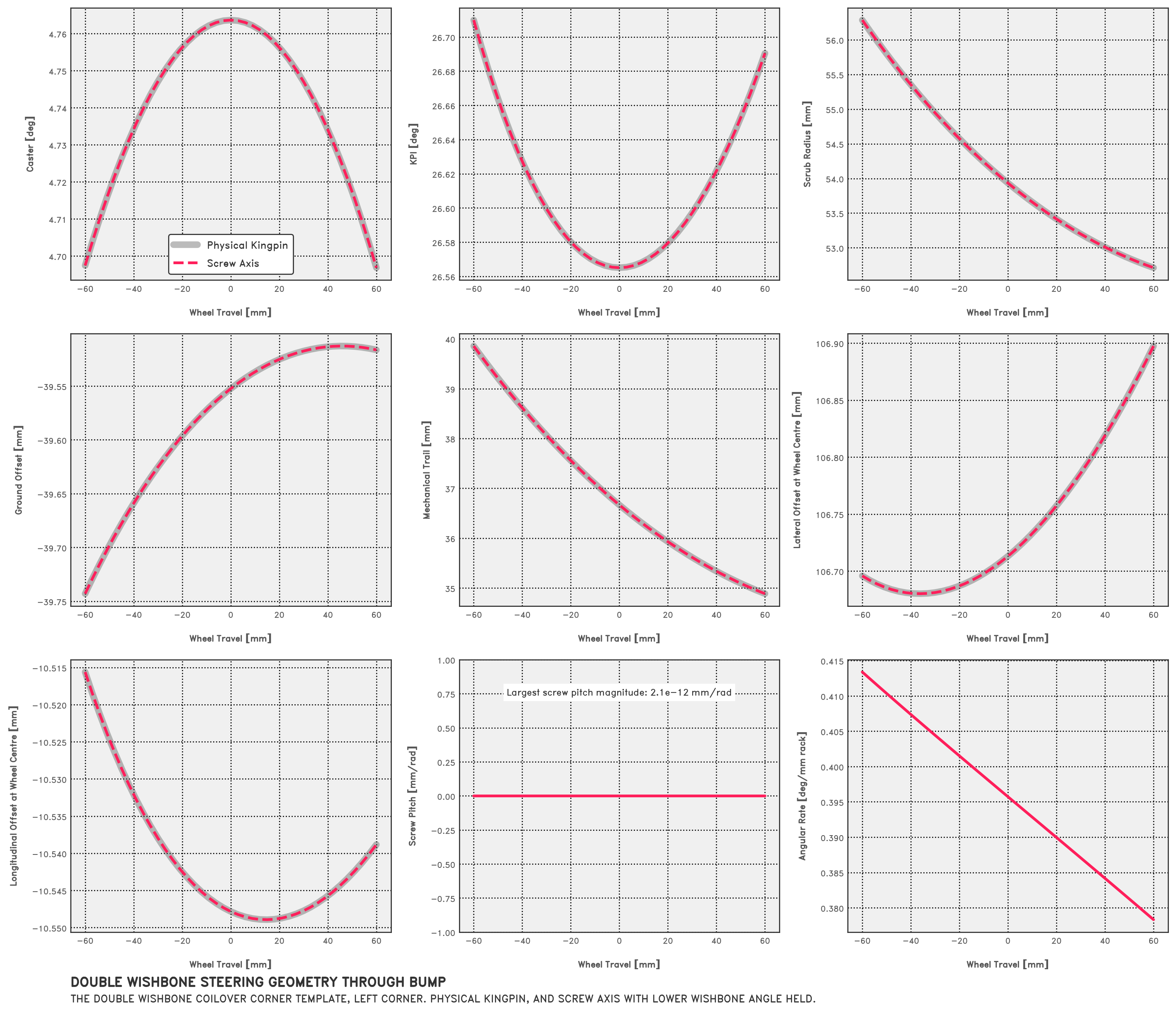
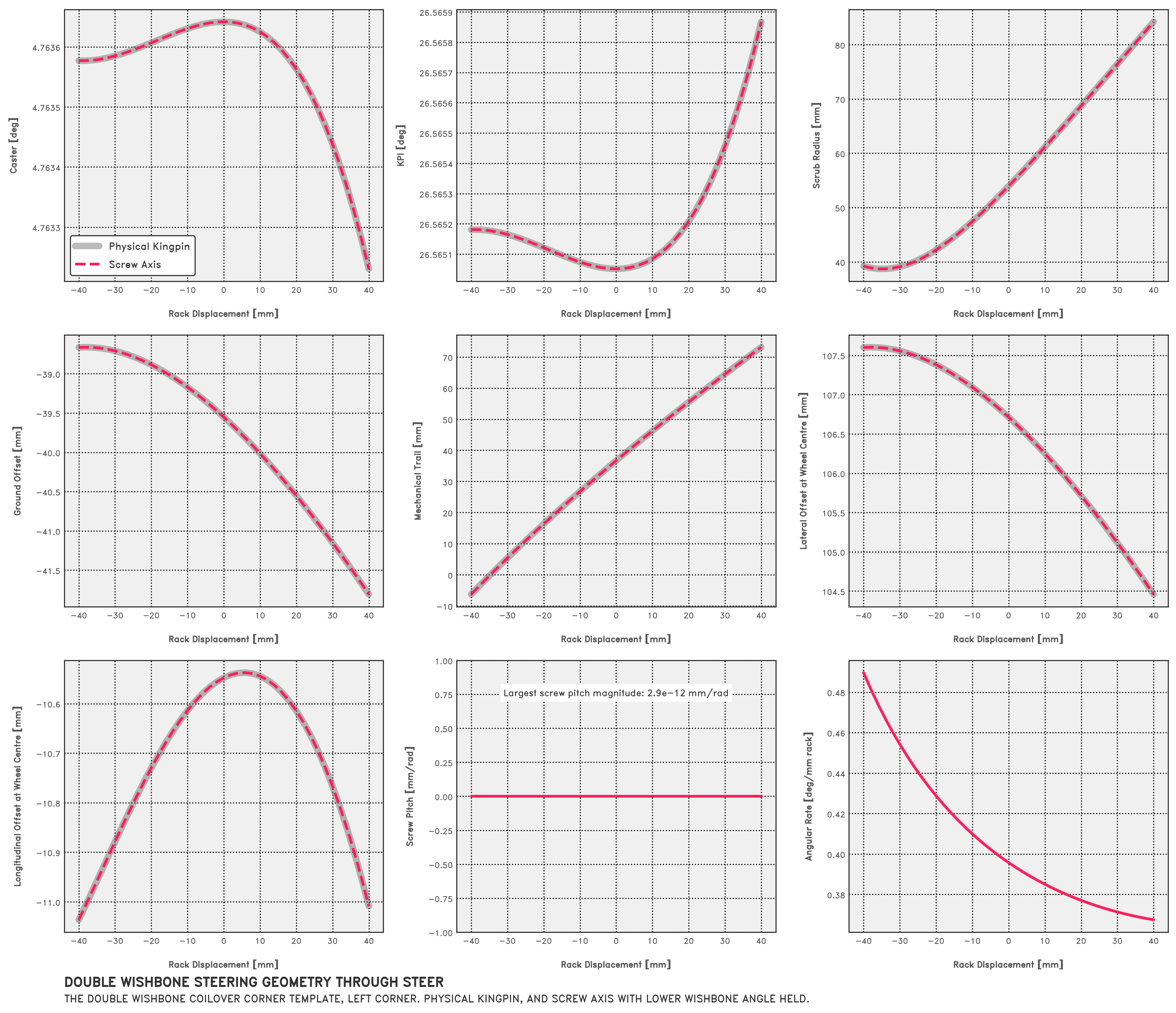
The two agree to within $6 \times 10^{-11}$ in each metric’s native units on both sweeps, and the pitch is zero to $3 \times 10^{-12}$ mm/rad, so the virtual axis is the kingpin, frame by frame. The one panel the physical kingpin can’t fill is the angular rate: the upright’s total rotation per millimetre of rack, which falls from 0.41 to 0.38 °/mm through bump and from 0.49 to 0.37 °/mm through the rack travel as the trackrod angle changes.
Isolating the steer response
With that in place, we can get point derivatives, fit a twist, turn it into a steer axis, and recover the double wishbone’s kingpin. We can now put numbers to the differences between the holds introduced earlier, and see how far a different hold can move the axis from the kingpin.
This part ended up needing more thought than the fitting itself… and I’m still not convinced I know exactly what I want.
Partial derivatives and what we ‘hold’
The screw axis fit has no idea what the supplied derivatives mean. It will fit any rigid motion of the upright, whether that’s bump, roll, or anything else, and it can’t tell whether that motion was steering.
The motion we get depends entirely on the target basis. $\partial q / \partial t_j$ is a partial derivative, which is only defined once the held quantities are fixed. That’s why our derivative with respect to rack displacement has to come with a hold: the held coordinates are part of the definition of the derivative, so changing them changes the result.
Why you don’t want to fix wheel centre height
The convenient choice would be to reuse whatever the sweep is holding. Our typical steer sweep drives the rack and holds wheel centre height constant, so the wheel doesn’t move up and down while it steers. We already have the point derivatives for that motion, so it would be easy enough to pass them straight to the fit.
However, that response generally doesn’t recover the kingpin axis. Steering about an inclined kingpin can raise or lower the wheel centre. If the sweep holds the wheel centre height fixed, the solver has to cancel the jacking with suspension travel. The point derivatives with respect to rack displacement then describe a mixture of steering and bump.
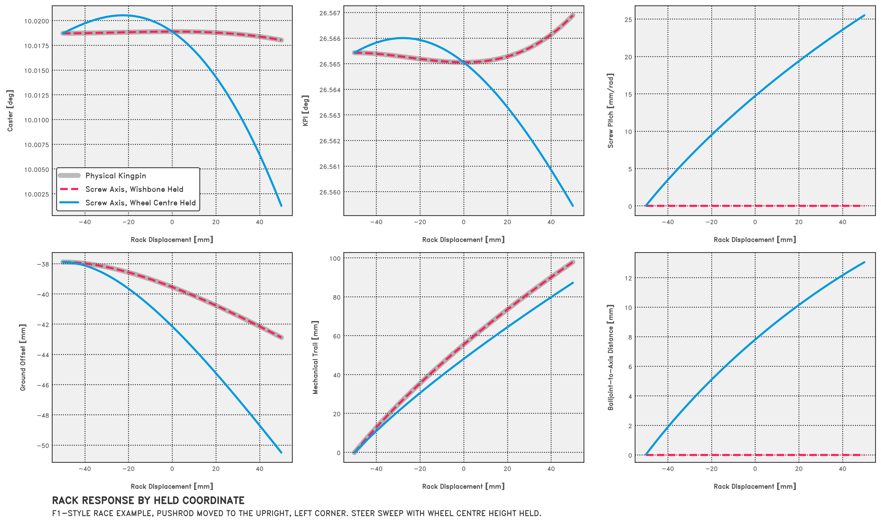
We can see this in the balljoint derivatives. At design condition on the F1 style example, the sweep’s own rack tangent moves both balljoints up at the same rate, 0.11 mm per mm of rack, with fore-aft and lateral components that are zero to numerical precision, while wheel centre height stays fixed. Away from that state, or with different wishbone geometry, the compensating motion can include more rotation. The core test suite checks this design-condition case from both sides on its own upright-pushrod fixture (test_wheel_center_height_control_does_not_contaminate_virtual_metrics): under the sweep’s own rack tangent, both balljoints share the same nonzero vertical rate while the wheel centre’s vertical rate is zero, and under the wishbone hold both balljoint rates are zero and the virtual metrics match the physical ones. The fit of the sweep’s tangent has correctly described the combined steering and bump motion, and the axis it gives doesn’t pass through the balljoints, as the figure below shows.
The way in which it differs from the kingpin is worth a closer look. At that design state, the equal balljoint derivatives make the compensating bump a pure translation of the upright to first order. Going back to the screw axis extraction, adding a translation per unit rack displacement $v$ to the twist leaves $\rho$, and so the axis direction, unchanged. It adds $\rho \cdot v / |\rho|^2$ to the pitch and moves the axis sideways by $\rho \times v / |\rho|^2$. Here $v$ is vertical and the kingpin is about 28° from vertical, so most of the jacking should show up as pitch, with the rest moving the axis sideways by the pitch times $\tan 28°$. At design condition, the two axes have the same direction to numerical precision, while the pitch is 14.7 mm/rad and the fitted axis sits 7.8 mm from the balljoints.
Through ±50 mm of rack travel on the F1 style example, the compensating motion remains close to a translation: caster and KPI differ from the physical kingpin by at most 0.017° and 0.007°, which would be very easy to miss. However, the pitch reaches about 25 mm/rad, the fitted axis sits up to 13 mm away from the balljoints, and ground offset and mechanical trail differ by up to 7.6 mm and 10.6 mm respectively. The angles look fine, but the axis position doesn’t recover the kingpin.
There’s another practical problem. Suppose we reach the same configuration in two different sweeps, one holding wheel centre height and one holding damper length. If we borrow each sweep’s targets, we’ll get different steering responses at the same configuration. I don’t want changing a sweep setup to quietly change what a steering metric means. We need to choose what we’re holding for that calculation, and keep that choice separate from the sweep which got us there.
What you might want to fix instead
Practically, the choice depends on the suspension layout. A double wishbone gives us an arm angle we can hold; other layouts need a different coordinate. In the code, each suspension type declares the choices it supports and which one to use by default.
For a double wishbone, the default is the lower wishbone angle, which we’ve already seen gives us pure rotation about the kingpin. That needn’t keep the inboard suspension still, though. With an offset upright-mounted pushrod, the rocker and damper can move during that rotation. The double wishbone model therefore also offers a damper-length hold where a damper is fitted. For the rocker arrangement used here, fixing that length locally fixes the rocker position: this is the ‘fixed internals’ experiment from earlier. It can require the wishbones to move, so it defines a different response from the default wishbone-angle hold. The double wishbone catalogue says as much: when the pushrod pickup is on the upright, the damper-length option is published with a warning (double_wishbone.py):
mounted_to_upright = self.actuation.moving_pickup_body == self.UPRIGHT_BODY
warning = (
    "Locks the internal suspension at its current damper length. "
    "Because the actuation pickup is mounted on the upright, the "
    "wishbones and hub may move in response to steering and the "
    "response axis may differ from the physical kingpin axis."
    if mounted_to_upright
    else None
)
With its pushrod moved onto the upright, the F1 style race example offers all three holds:
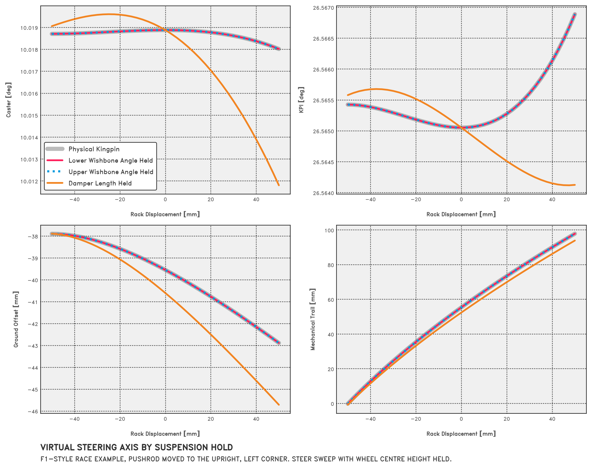
The two wishbone-angle holds agree with the physical kingpin, and with each other, to numerical precision. Holding damper length instead barely changes the angles (caster and KPI shift by at most 0.006° and 0.003°), but it does move the axis, by up to 2.8 mm of ground offset and 4.0 mm of trail, with pitch between 1.2 and 9.5 mm/rad. This is the same pattern as with wheel centre height held, though on this geometry it’s the smaller of the two effects. This is why the hold is a setting in the app, under ‘Virtual Steering Response’ in the sweep profile, rather than a solver default: it can change the numbers we’d use to compare two layouts.
The coilover template from the previous section is different: there, holding damper length also recovers the kingpin. The coilover is mounted on the lower wishbone, so fixing its length locally fixes that arm. The separation here comes from the upright-mounted pushrod, whose pickup can move during steering even with the wishbones held.
Multi-link metrics
Now that we can recover both the double wishbone’s kingpin and its steering metrics, and we’ve seen what the hold does, we can use the same process for our multi-link.
Multi-link: fixed damper length
There isn’t a wishbone hinge angle to hold here, so the coordinate we currently use is installed damper length. It’s the only option the multi-link model offers at present. That sounds straightforward enough, but the damper pickup can itself move as the upright steers.
The whole catalogue is one option, from MultiLinkSuspension.suspension_hold_catalog in multi_link.py:
return SuspensionHoldCatalog(
    default_option_id="damper_length",
    options=(
        SuspensionHoldOption(
            id="damper_length",
            label="Damper length",
            description=(
                "Locks the internal suspension at the current installed "
                "true damper length during the steering response. A "
                "multi-link corner has no physical kingpin, so the "
                "resulting screw axis is the definition of its steering "
                "axis under this locked-internals condition."
            ),
            hold=CoordinateHold((damper,)),
        ),
    ),
)
In the test geometry, that pickup is fixed to one of the lower links, as shown in the annotated screenshot of Suspension Explorer below.
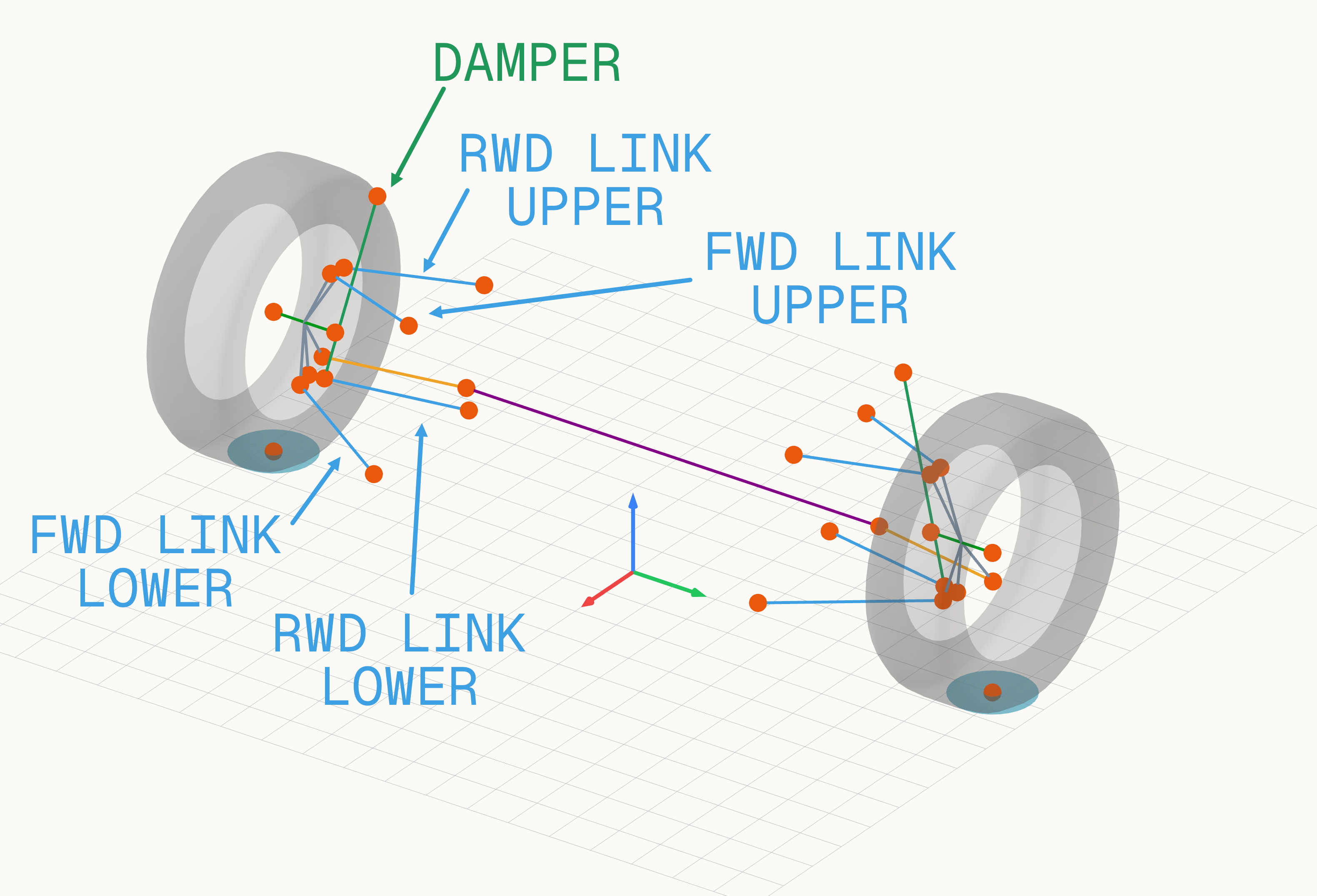
That link moves during steer, and holding damper length forces the rest of the mechanism to accommodate it. A pickup carried by the upright would introduce the same sort of coupling, as with the F1 style pushrod above, though the multi-link model can’t mount one there yet. We’ve fixed the damper length, but the links are still free to move, and some compensating suspension motion is part of the response we’re measuring. How much depends on the layout and where the pickup sits.
The multi-link test geometry was built around the designed axis from earlier: all four locating-link lines pass through it, so at design condition the link-pair construction sits on that axis, and the only thing pulling the screw axis off it is the damper hold. Pure rotation about the designed axis would increase damper length by about 0.0125 mm per millimetre of rack displacement, so holding that length requires compensating suspension motion. That coupling is why the screw axis doesn’t land exactly on the designed axis: KPI comes out 0.05° lower than the link-pair construction, ground offset differs by 0.4 mm, and there’s a small pitch of −1.2 mm/rad.
Through bump and steer
We fit the axis to the steering response with damper length held, then pass it to the same metric functions. Here, the virtual family is the only one reported, since there’s no physical axis to compare against.
Away from design condition, the paired link lines also stop meeting, which is the problem we flagged earlier: the shortest distance between the two lower link lines grows to 4 mm over ±60 mm of bump, and both pairs are around 5 mm apart at ±40 mm of rack. The virtual balljoints become the midpoints of a gap rather than intersections, and this is on a geometry that was designed to suit the construction.
The figure below shows the full set for the multi-link test geometry through ±60 mm of bump, with the link-pair construction evaluated by the same metric functions for comparison:
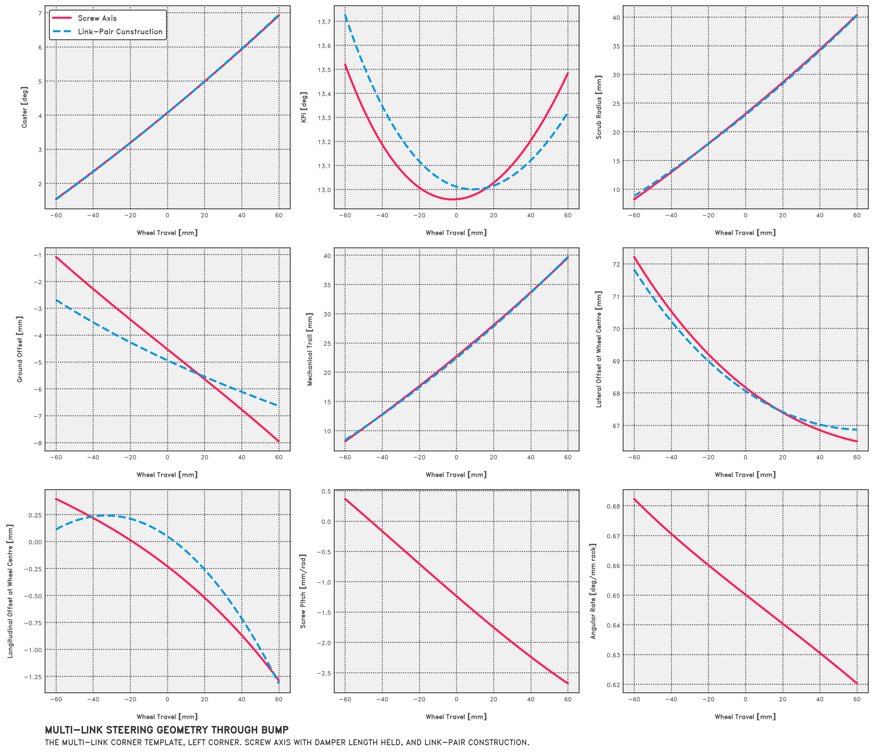
Caster and trail from the two methods track each other closely, but KPI and ground offset don’t; by the ends of the bump travel, the link-pair construction differs from the response with damper length held by up to 0.2° of KPI and 1.6 mm of ground offset. The pitch stays small (−2.7 to 0.4 mm/rad), and the total upright angular rate with respect to rack travel falls from 0.68 to 0.62 °/mm of rack as the wheel moves up.
At design condition in this multi-link example, the total angular rate with respect to rack travel is 0.650°/mm, while the derivative of wheel heading with respect to rack displacement has magnitude 0.632°/mm under the same damper-length hold.
Through ±40 mm of rack, which takes the wheel to roughly ±26° of steer:
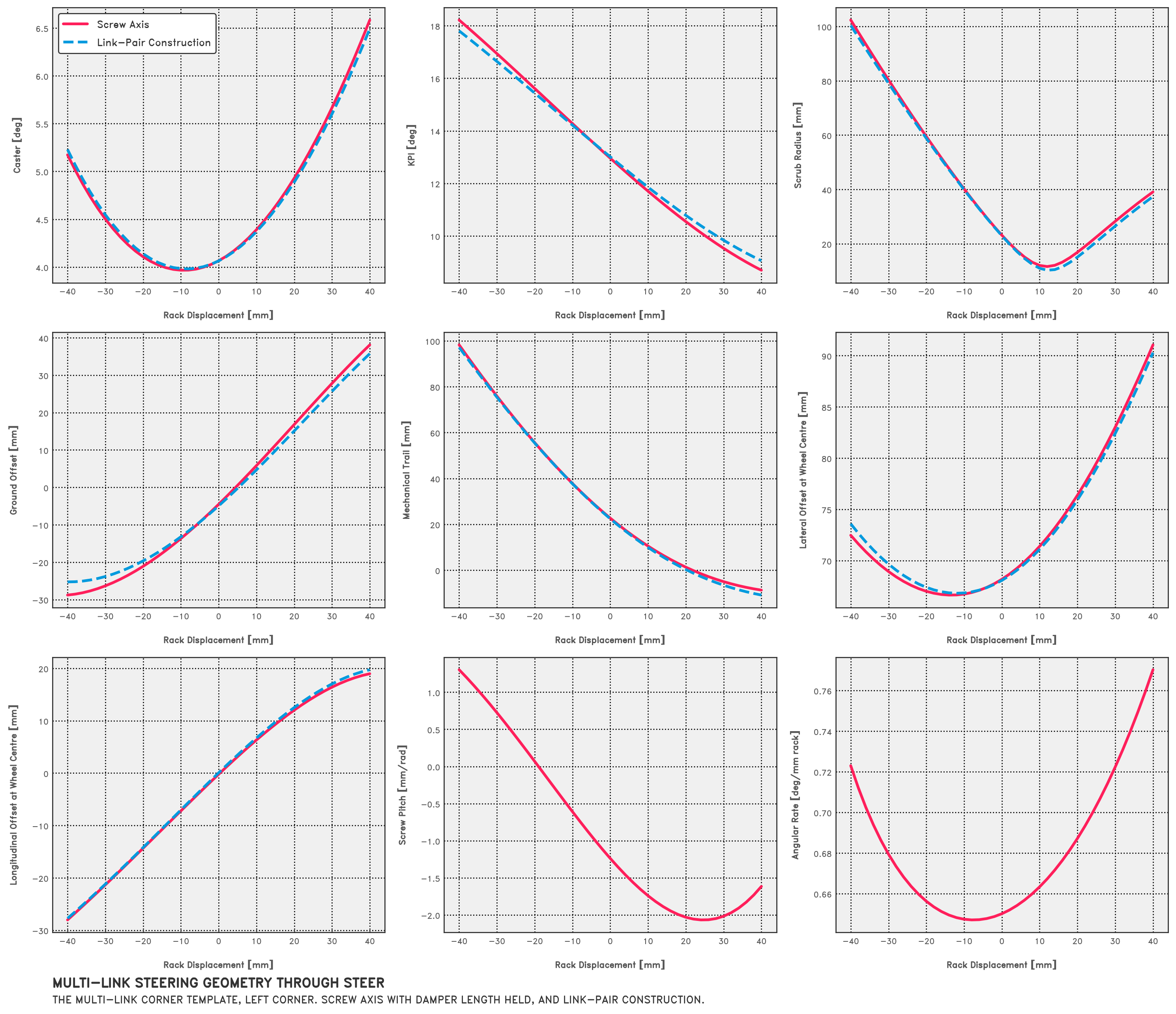
Here, the gap grows to 0.4° of KPI and 3.5 mm of ground offset at full lock. None of these differences are huge, but I suspect they’re large enough to matter when comparing layouts. We do have to remember what we’re comparing: the red curve includes the suspension motion needed to hold damper length. Move that pickup and we can change the response, even with the same locating links. The link-pair construction has no way to account for that choice.
Steer axis migration
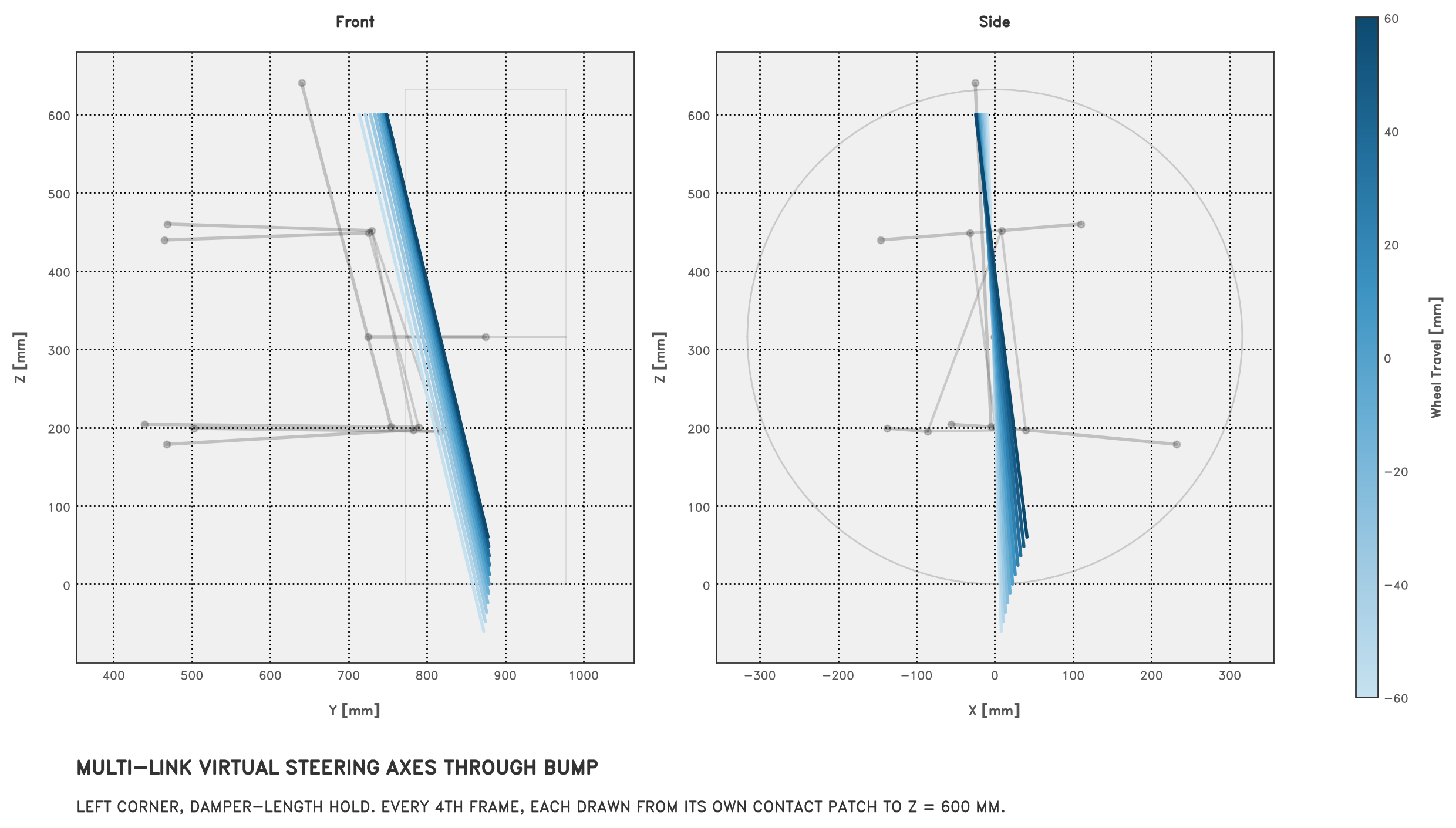
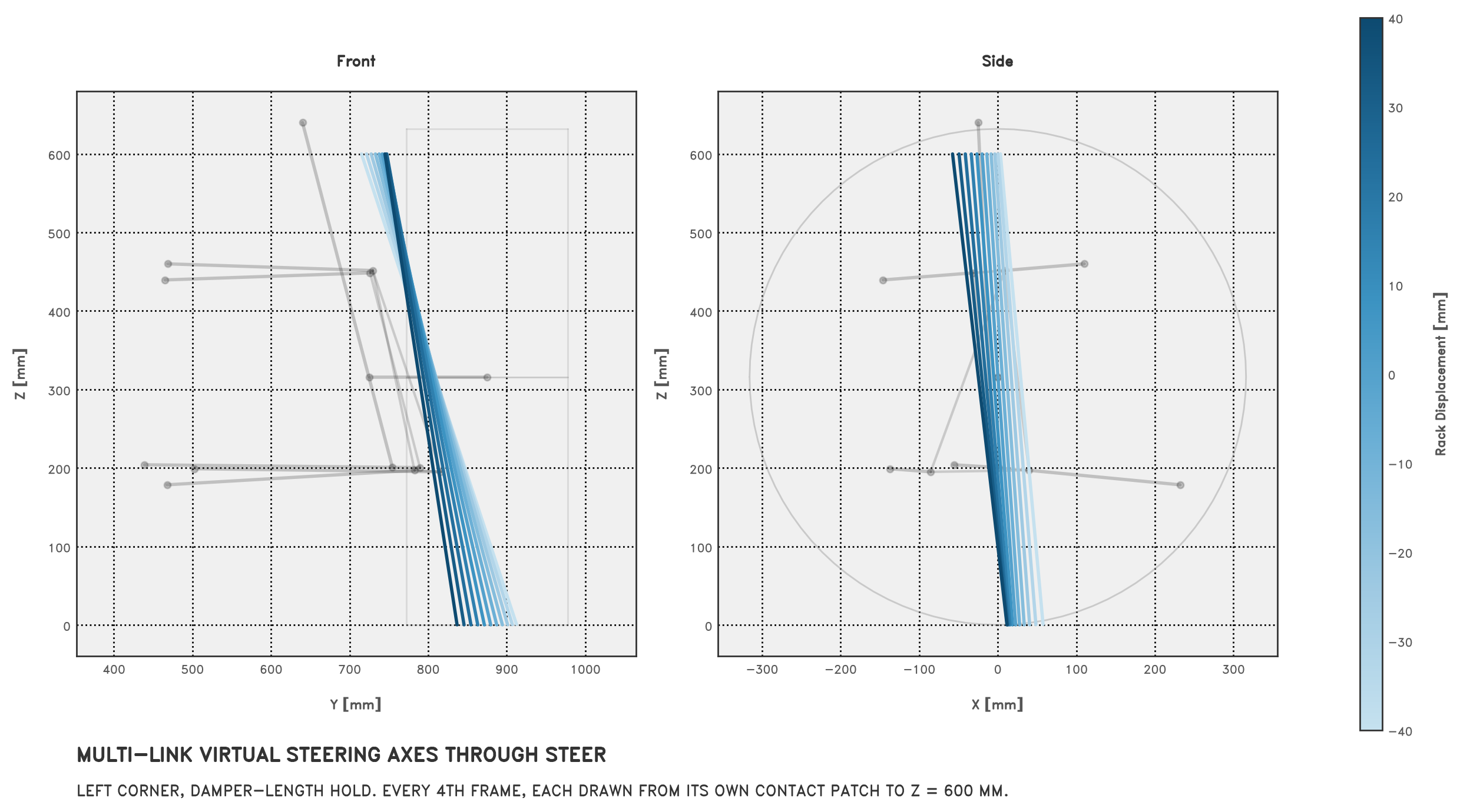
I also find it useful to draw the axes themselves. We have one steering response axis at each solved position, so we can put them all on the same plot and see how the virtual kingpin moves through travel. Taken together, those axes form a ruled surface. A surface traced by the instantaneous screw axes of a body’s actual motion is called an ‘axode’; the distinction between that motion and our steering response matters here.
To read these plots, imagine pausing the suspension at each step of the sweep, holding its current damper length, and interrogating how it would move if we perturbed the rack. Each line is the axis for that steering movement. The bump sweep itself holds the rack, while the steer sweep holds wheel centre height, so the axes describe a different motion from the one carrying us between steps. That’s why these surfaces aren’t the axodes of the sweep motion.
Each axis comes directly from the derivatives with respect to rack displacement at that position; we don’t difference neighbouring frames or fitted axes. On a double wishbone with a wishbone angle held, we already know each axis will pass through the current balljoints. The multi-link plot is more useful because we don’t have those two physical points to guide us. Each line is drawn from its own contact patch height up to 600 mm, so in the bump plot the lower ends fan out with the wheel travel.
Through bump, the axis is mostly carried along with the upright, tilting rearward as caster increases:
Through steer, the axis swings visibly in both views; this is where the KPI and caster ranges in the steer metrics above come from:
The app can also show the steering axes and their traces alongside the moving linkage:
Further work
This gives us a multi-link corner we can solve, and steering metrics we can compare through travel, provided we’re clear about what we’re holding. There are still a few things I’d like to add:
- Instant centres for multi-link. The current front and side view instant centres come from intersecting wishbone planes. A multi-link has no wishbone planes, so they’re undefined, and the swing arm and anti metrics that depend on them come back as nulls. I’d like to try reusing the derivative calculation with bump as the input, then work out what useful front and side view equivalents we can extract. Projecting the spatial screw axis alone won’t generally give us a planar instant centre, particularly if the motion has nonzero pitch or an out-of-plane component, so there’s some geometry left to think through there.
- More holds for multi-link. Damper length is the only option at the moment. A hold based on the link geometry rather than the damper, e.g., the elevation of one of the lower links, would let us keep the same definition when we move a damper pickup. I’d be interested to see how much difference that makes across a few layouts.
- A contact patch or ‘wheel centre on ground’ hold. If you sit a real car on the ground and cycle the rack, nothing holds a wishbone angle or a damper length fixed. The vertical constraint is really that the tyre stays on the ground, and everything else is free to move. We don’t have a tyre model, but holding the wheel’s centre plane point on the ground could be a reasonable proxy for that. Like the wheel centre hold, it would fold the jacking effect from an inclined steer axis into the response as suspension travel, so it generally won’t give back a double wishbone’s kingpin axis. However, here, that motion is probably OK; it’s how the upright moves when the car is steered on the road rather than an artifact of how the sweep was set up.
Aside: why the centroid?
The code uses the centroid of the fitted points as $p_{ref}$. The centroid decouples the translational and rotational parts of the fit, and the rotational part has the form of a rigid-body inertia relation.
The normal equations for the fit are $A^\top A x = A^\top b$. Using $[d]_\times^\top = -[d]_\times$:
$$ A^\top A = \begin{bmatrix} n_p I_3 & -\left[\sum_i d_i\right]_\times \\ \left[\sum_i d_i\right]_\times & \sum_i [d_i]_\times^\top [d_i]_\times \end{bmatrix} $$If $p_{ref}$ is the centroid, then $\sum_i d_i = 0$ and the off-diagonal blocks vanish, so the fit splits into two independent problems:
$$ r_{ref} = \frac{1}{n_p} \sum_i r_i, \qquad \underbrace{ \left( \sum_i \left(|d_i|^2 I_3 - d_i d_i^\top\right) \right) }_{\mathcal{I}} \rho = \sum_i d_i \times r_i $$The first says that the reference point derivative is the average point derivative. The second is a little more interesting: the matrix $\mathcal{I}$ on the left is the inertia tensor of a set of unit point masses located at the fitted points. The right-hand side has the algebraic form of angular momentum $L$ about the centroid. So the fitted angular rate with respect to rack travel has the same form as $\rho = \mathcal{I}^{-1} L$ for a rigid body with that mass distribution. This is an analogy between the equations; our inputs remain position derivatives with respect to rack displacement.
The same analogy explains the failure conditions. An inertia tensor is singular when all of the mass lies on a line, since there’s zero moment of inertia about that line. Likewise, if all the fitted points are collinear, rotation about the line they lie on doesn’t move any of them, so it can’t be observed. We need at least three non-collinear points for $A$ to have full rank.