Building a suspension kinematics tool | Part II
Shims and solvers: SymPy, analytical Jacobians, and automatic differentiation.
Contents:
Introduction
This post is the second in a series on building a tool to simulate the kinematics of a racing car’s suspension.
The first post walked through the earliest stages of building a tool of this kind. It covered a couple of ways to go about solving this kind of problem, introduced the concept of geometric constraints, explained the requirement for an iterative solve and the utility of Newton’s method, and walked through the assembly of a system which could actually solve for the positions of all the points in a suspension layout during combined bump and steer sweeps.
However, we did not cover all the important parts of a system like this…
What we’ve still got to build
The previous post was tied to a tagged release of open-kinematics
at v0.1.0. At this version, we had not yet really considered:
- Setup options.
- To accommodate relevant setup parameters commonly adjusted in a motorsport setting (ride height, camber, toe, etc.), the tool must support configuration options relating to shim/turnbuckle adjustments.
- Solver improvements.
v0.1.0used a Levenberg-Marquardt solver with out-of-the box numerical gradient estimation. A more considered approach to Jacobian assembly should offer improvements to derivative accuracy and solve performance.
- Metrics.
- To be useful, the tool will require interrogable outputs for camber, caster, toe, antis, RCH etc.
All of these items should be soluble, and once we’ve delivered those, we’ll be well on our way to having built something that might actually be useful.
Relative to last time, this post should involve a bit less maths, a bit less $\LaTeX$, and less directed acyclic graphs. Instead, we’ll be focusing on some numerical methods and scientific computing adjacent wizardry, building secondary solves, and starting to think about the squiggly lines the vehicle dynamicists want from us.
Setup options: on outboard camber shims and pre-solve solves
Last time, I noted that outboard camber shims are a slightly awkward setup item to deal with in a tool like this. This is because camber shim changes cannot be dealt with in quite the same way as something like a rack position or balljoint position move, where we keep the geometry of each component fixed and ask the solver to find a new pose.
The image below shows the sort of thing I mean here. In this image of an old Caterham F1 car’s rear upright, you can see that we could make camber more positive by adding shim between the shim block and the main upright body, and we could make camber more negative by removing shim.
When we adjust the shim stack here, it’s not just a case of moving the assembly to another position; the geometry of the upright itself changes, and the positions of the axle points and any other attachments on the upright change with it. The camber block is free to rotate about the UBJ, while the rest of the upright body is free to rotate about the lower balljoint to accommodate the shim thickness change. Beyond that, you might need one or both of the wishbones to rotate about their axes in order to keep the shim stack contacting faces of the camber block and upright body both aligned and parallel†. So, before we solve any bump or steer steps, we first need to work out the geometry of the shimmed upright.
In reality, this step serves to take the nominal geometry of the suspension, then apply a pre-simulation solve to determine what the actual as-shimmed geometry looks like. It’s not quite a ‘solve within a solve’ situation, but it is necessary to get the geometry right before we can even start the main sweep.
†This point in particular I did not appreciate until I’d had a first attempt at modelling this behaviour. See the two shim solve sections below for more details.
Shim solve concept: V1
My first attempt at this, I realised as I was writing this post, did not capture the full effect of the shim change. It’s in broadly the right ballpark, but we’re basically making a small-angle approximation assumption here that we can avoid by doing a better job. However, I thought I’d leave this in here to show how this sort of thing comes together…
For the style of camber block arrangement shown above, the relevant inputs are:
- The design position of the shim face centre, $p_{shimFaceCenter}$,
- The shim face normal, ${n}_{shimFace}$,
- The design condition shim thickness, $t_{shimDesign}$,
- The setup condition shim thickness, $t_{shimSetup}$.
In terms of what these look like, $p_{shimFaceCenter}$ is just a three-element coordinate vector, ${n}_{shimFace}$ is a unit vector pointing out from the shim face, and $t_{shimDesign}$ and $t_{shimSetup}$ are scalar thickness values.
With that setup, thickness change is simply:
$$ \Delta t_{shim} = t_{shimSetup} - t_{shimDesign} $$So, the shim face wants to move by $\Delta t_{shim}$ along ${n}_{shimFace}$, giving a shim offset vector:
$$ v_{shimOffset} = \Delta t_{shim} {n}_{shimFace} $$Here, because both the upper and lower balljoints remain in place, and chassis-mounted points obviously remain in place, what changes is the rigid body hanging off the shimmed part of the upright: the axle points, and any other configured upright-mounted attachments.
So the actual job is to find the rotation of that body about the lower balljoint which carries the shim face centre from its design position to its setup position.
If we let $p_{lowerBalljoint}$ be the lower balljoint position, then we can assemble vectors from the lower balljoint to the shim face centre in both its design and setup positions:
$$ v_{lbjToShimDesign} = p_{shimFaceCenter} - p_{lowerBalljoint} $$$$ v_{lbjToShimSetup} = (p_{shimFaceCenter} + v_{shimOffset}) - p_{lowerBalljoint} $$The rotation axis is the normalised cross product of these two vectors (where $\operatorname{normalize}(v) = v / \lVert v \rVert$):
$$ u_{rotationAxis} = \operatorname{normalize}\left( v_{lbjToShimDesign} \times v_{lbjToShimSetup} \right) $$And the desired rotation angle is then the angle between those two vectors:
$$ \theta_{rotation} = \angle(v_{lbjToShimDesign}, v_{lbjToShimSetup}) $$If the cross product vanishes, the two vectors are parallel and no rotation is required. Otherwise, once we have $u_{rotationAxis}$ and $\theta_{rotation}$, the rest is just Rodrigues’ formula applied to every point that should move with the shimmed part of the upright.
Conceptually, the flow is roughly:
positions = hardpoints.copy()

offset = normalize(shim_normal) * (setup_thickness - design_thickness)
axis, angle = rotation_from_shim(lower_ball_joint, shim_face_center, offset)

rotate(axle_inboard, about=lower_ball_joint, axis=axis, angle=angle)
rotate(axle_outboard, about=lower_ball_joint, axis=axis, angle=angle)
rotate(any other upright-mounted points, about=lower_ball_joint, axis=axis, angle=angle)
open-kinematics packages this up inside DoubleWishboneSuspension.initial_state(). It copies the design hardpoints,
applies apply_camber_shim() if a shim config is present, recomputes any derived points, and only then builds the
SuspensionState.
Real-world implementation
Practically, for our double wishbone setup, the entire shim application logic is laid out like this:
@dataclass
class DoubleWishboneSuspension(Suspension):
...
    def apply_camber_shim(self, positions: dict[PointID, np.ndarray]) -> None:
        """
        Apply camber shim transformation to attachment positions.

        The shim rotates only attachments (axle points), not the hardpoints
        (ball joints).
        """
        if self.config is None or self.config.camber_shim is None:
            return

        shim_config = self.config.camber_shim

        # Build upright from current positions.
        point_ids = self.UPRIGHT_MOUNT_ROLES
        hardpoints = {pid: make_vec3(positions[pid]) for pid in point_ids.values()}
        attachments = {
            "axle_inboard": make_vec3(positions[PointID.AXLE_INBOARD]),
            "axle_outboard": make_vec3(positions[PointID.AXLE_OUTBOARD]),
        }
        upright = Upright.from_hardpoints_and_attachments(
            point_ids, hardpoints, attachments
        )

        # Compute shim offset.
        shim_offset = compute_shim_offset(shim_config)

        # Get shim face center at design (already a Vec3).
        shim_face_center_design = shim_config.shim_face_center

        # Lower ball joint is the pivot.
        lower_ball_joint = make_vec3(positions[PointID.LOWER_WISHBONE_OUTBOARD])

        # Compute rotation.
        rotation_axis, rotation_angle = compute_upright_rotation_from_shim(
            lower_ball_joint,
            shim_face_center_design,
            shim_offset,
        )

        # Apply shim to upright.
        upright.apply_camber_shim(lower_ball_joint, rotation_axis, rotation_angle)

        # Update positions with rotated attachments.
        positions[PointID.AXLE_INBOARD] = np.array(
            upright.get_world_position("axle_inboard")
        )
        positions[PointID.AXLE_OUTBOARD] = np.array(
            upright.get_world_position("axle_outboard")
        )

        # Rotate trackrod if it's upright-mounted.
        upright_mounted = self.config.upright_mounted_points
        if upright_mounted and "trackrod_outboard" in upright_mounted:
            trackrod_pos = make_vec3(positions[PointID.TRACKROD_OUTBOARD])
            trackrod_rotated = rotate_point_about_axis(
                trackrod_pos, lower_ball_joint, rotation_axis, rotation_angle
            )
            positions[PointID.TRACKROD_OUTBOARD] = np.array(trackrod_rotated)
With rotation logic as follows:
def compute_upright_rotation_from_shim(
    lower_ball_joint: Vec3,
    shim_face_center_design: Vec3Like,
    shim_offset: Vec3,
) -> tuple[Vec3, float]:
    """
    Compute the rotation axis and angle for the upright given a shim offset.

    The upright rotates about an axis through the lower ball joint. The rotation
    is determined by the constraint that the shim face center must move by the
    shim offset vector.

    The rotation axis is perpendicular to both:
    - The radial vector from lower ball joint to shim face center
    - The shim offset direction (parallel to shim normal)

    This means the axis is also perpendicular to the shim normal, which makes
    physical sense: pushing the shim face outboard causes rotation about an axis
    perpendicular to that push direction.

    Args:
        lower_ball_joint: Position of the lower ball joint (rotation pivot).
        shim_face_center_design: Design position of the shim face center.
        shim_offset: Offset vector from shim thickness change (parallel to shim normal).

    Returns:
        Tuple of (rotation_axis, rotation_angle_rad).
        rotation_axis is a unit vector through the lower ball joint.
        rotation_angle_rad is the angle to rotate the upright.
    """
    # Coerce to Vec3 (handles Pydantic model fields which may be typed as Vec3Like).
    shim_center = coerce_vec3(shim_face_center_design)

    # The shim face must move to: shim_face_center_design + shim_offset.
    shim_face_target = make_vec3(shim_center + shim_offset)

    # Vector from lower ball joint to design shim face center.
    r_design = make_vec3(shim_center - lower_ball_joint)

    # Vector from lower ball joint to target shim face center.
    r_target = make_vec3(shim_face_target - lower_ball_joint)

    # The rotation axis is perpendicular to both r_design and r_target.
    # Note: r_target = r_design + shim_offset, so by cross product properties:
    #   r_design × r_target = r_design × (r_design + shim_offset)
    #                       = r_design × shim_offset
    # Therefore the axis is perpendicular to both the radial arm and the shim normal.
    cross = np.cross(r_design, r_target)
    cross_magnitude = np.linalg.norm(cross)

    if cross_magnitude < EPSILON:
        # Vectors are parallel - no rotation needed.
        return make_vec3(np.array([0.0, 0.0, 1.0])), 0.0

    rotation_axis = make_vec3(cross / cross_magnitude)

    # Compute the rotation angle between the two radial vectors.
    rotation_angle = compute_vector_vector_angle(r_design, r_target)

    return rotation_axis, rotation_angle
Note that sequencing is also important here. The geometric constraints are constructed from initial_state(), so the
link lengths and upright angle targets are taken from the already-shimmed geometry. In other words, the main sweep solve
setup does not carry any kind of separate shim residual, nor does it run an inner nonlinear solve to discover the
shimmed pose. By the time the main solver starts iterating, the shimmed suspension is simply the suspension.
Comparison
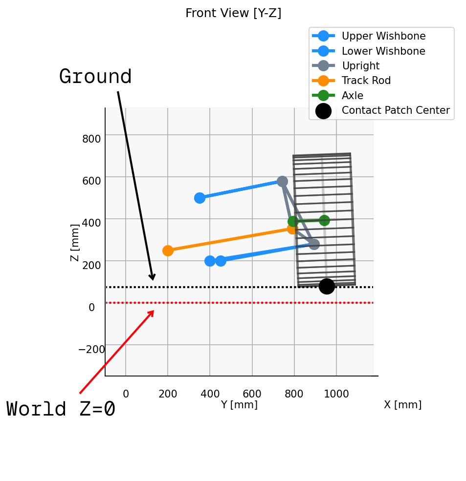
The plot below shows a front view of a given suspension setup with only one change: an intentionally extreme 30mm delta in camber shim. The blue series show the design condition setup, with 30mm of camber shim, and red shows the same setup but with the camber shim removed.
What can be seen here is that all the wishbone points, inboard and outboard, remain in the same place. However, the upright mounted points, i.e., the axle endpoints and the outboard trackrdo pickup, have moved in a way consistent with the rotation we would expect from the shim change.
For a bit more detail, see these two:
†Note that we indicate both ‘wheel centre on ground’ and ‘contact patch’ here. Later in this post, we discuss approach to ground planes and end up removing the ‘wheel centre on ground’ concept entirely; something to be revisited in a later post.
Shim solve concept: V2
Where V1 went wrong
If you missed the shortcomings of the method above, hopefully this diagram will help. Practically, what I was doing was assuming a fixed shim normal direction and just moving the shim face along that normal by the thickness change, then rotating the upright to accommodate that. We were also applying a constraint to the system that didn’t exist; forcing the balljoints to remain a fixed distance apart, which is not actually the case in a real shim change. We were both simplifying the problem and mischaracterising its nature.
In reality, the camber block is free to rotate about the top balljoint, so as we add more shim and the upright body rotates out and down, the camber block will also rotate, with the shim normal rotating with it. The top wishbone itself is also free to rotate about its inboard axis, and we need to account for that.
The figure below shows what I mean. Using Onshape’s sketch constraints (and presumably thus D-Cubed’s geometric constraint solver), it shows the effect of reducing shim thickness on the direction of the shim face normal. In both plots, the idea is that we have a simplified front-view of an upright with wheel/tyre and a camber block type adjustment. The upright body is highlighted in blue, with the balljoints marked in red.
If we take a closer look at the figure, you can see that in the design condition plot on the left hand side, the shim normal is noticeably closer to the horizontal than it is on the right hand side, where the shim thickness has been reduced.
In our V1 approach, we did not account for this. We computed the shim normal at the design condition, then just moved the shim face along that normal by the thickness change. In reality, as the upright rotates, the shim normal also rotates, and the shim face moves along that new normal direction. This means the actual path of the shim face centre is not a straight line along the original normal, but rather an arc that follows the rotation of the upright.
A better way
So, instead of making poor assumptions on shim face movement, we can lean on the solver machinery a little bit more.
What we have in this setup is effectively a very limited set of geometric constraints. Rather than guessing a shim face translation directly, we can treat the split upright as a small constrained mechanism and let a local least-squares solve find the pose which satisfies the shim thickness, face alignment, and trackrod geometry. If we look at the Lotus upright again, it’s basically been cleaved in two, and we care only about the points about which either half can rotate (the LBJ and the UBJ), the faces which will actually contact the shim stack, and the trackrod which stops the whole upright from ‘steering’.
https://www.eliseparts.com/shop/genuine-br-lotus-parts-1/camber-shims/
Drawing out what we need here in Onshape again, we can iron out the constraints we really need. Looking something like front-on, this plot shows that we can achieve controlled camber change by changing shim thickness, provided the following assumptions hold:
- The camber block is free to rotate about the upper ball joint.
- The main upright body is free to rotate about the lower ball joint.
- The shim stack contacting faces remain parallel to each other.
- The shim stack contacting faces remain aligned, and are not free to rotate about any axis normal to their surface.
- The parallel distance between the shim faces is equal to the thickness of the fitted shim.
- The lower wishbone and lower balljoint are fixed in place.
- The upper balljoint is free to move according to the motion allowed by the rigid wishbone.
- The trackrod is of fixed length and remains attached to the upright and the (fixed) rack.
This plot shows the effect of reducing camber shim thickness on camber. Practically, as shim is reduced, the upright body, carrying the axle, rotates clockwise about an axis running through the lower balljoint and normal to the view plane. To accommodate this, the top wishbone rotates anticlockwise about its inboard axis, and the camber block pivots to keep the shim faces parallel and contacting the shim stack.
Constraints and degrees of freedom
More completely, the degrees of freedom available to us here are:
- $\theta_{uwb}$, the upper wishbone rotation angle. 1 DOF.
- $\rho_{camberBlock}$, the camber block rotation vector about the upper balljoint. 3 DOF.
- $\rho_{uprightBody}$, the lower upright body rotation vector about the lower balljoint. 3 DOF.
From a given set of these values, we can compute the positions of all the points in the system.
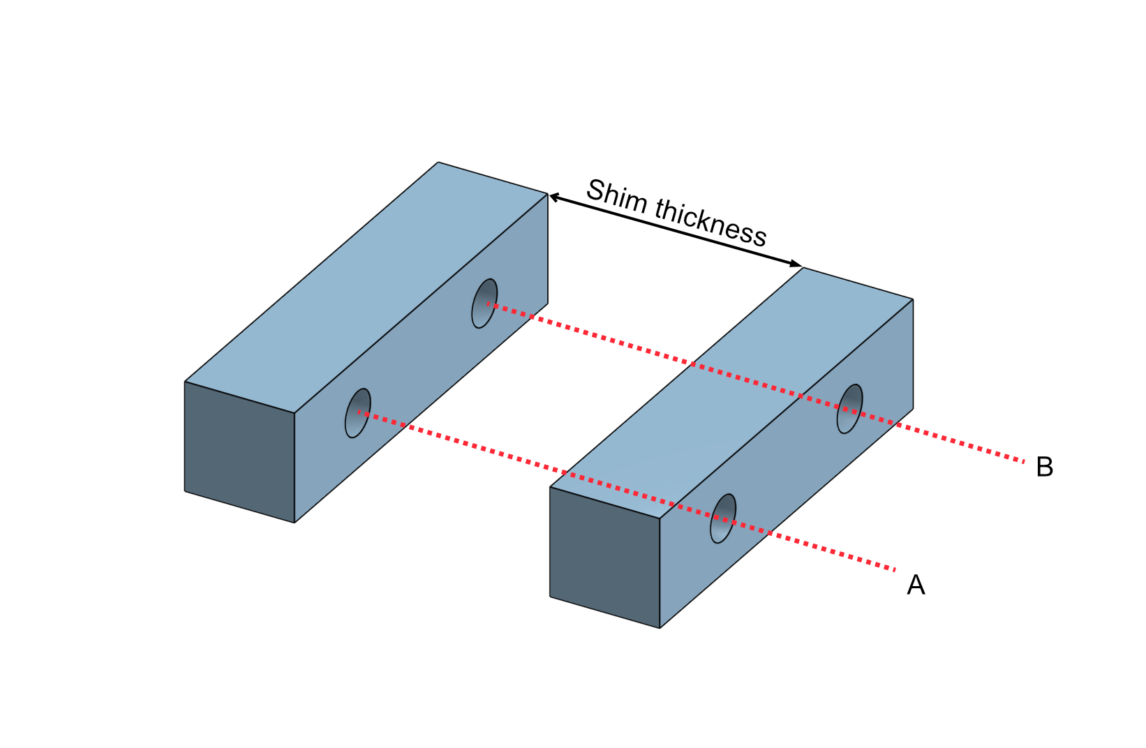
To properly describe the constraints, we first introduce the concept of ‘datum points’; a pair of imaginary points on each shim contacting face. In the implementation, these are configured as two ordered points in the mid plane of the design condition shim, which are offset by $\pm 0.5 t_{design}$ along the face normal to recover the camber block and upright body shim face datum positions. Each point, $A$ and $B$, has a corresponding point on the opposite face. These are intended to model something like dowelled connection between the two faces, dictating that both the camber block and the upright body shim faces remain parallel to one another, but cannot rotate relative to one another about any axis normal to those faces.
The figure below shows what I mean. The centre of each hole on the shim contacting face represents either $A$ or $B$, and we force an axis through those points. Then, the camber block and upright body can move along this axis pair, preventing relative rotation between faces, but maintaining parallelism between the faces across a range of shim thicknesses.
With that out of the way, the implementation is trying to drive four geometric conditions to zero:
Datum point A ‘closure’. The vector from the camber block’s first datum point to the upright body’s first datum point must be equal to the fitted shim thickness taken along the upper face normal:
$$ p_{uprightBodyA} - p_{camberBlockA} - t_{setup}{n}_{camberBlock} = 0 $$Because that’s a 3D vector equality, it contributes 3 scalar residuals.
Datum point B closure. The same condition is imposed at the second datum point, B:
$$ p_{uprightBodyB} - p_{camberBlockB} - t_{setup}{n}_{camberBlock} = 0 $$This contributes another 3 scalar residuals. Using two datum points rather than one stops the faces satisfying the thickness condition at one point while still being clocked incorrectly relative to each other.
Face normal alignment. The upper and lower shim contact faces must point in the same direction:
$$ {n}_{uprightBody} - {n}_{camberBlock} = 0 $$This is another 3-component vector equality, so it contributes 3 scalar residuals. It prevents the solver accepting a state where the faces are separated correctly but tilted relative to one another.
Trackrod length preservation. The trackrod is treated as a rigid link with a fixed inboard position (at the rack), so its length must remain equal to the design condition:
$$ \lVert p_{trackrodOut} - p_{trackrodIn} \rVert - L_{trackrod} = 0 $$This contributes 1 scalar residual. Without it, the split upright could try to satisfy the shim face conditions by changing roadwheel angle.
So, in total, this local solve has 10 scalar residuals. Those are the actual residual terms assembled in
compute_camber_shim_assembly_residuals().
Then, to actually compute our pose, if we let ${a}_{uwb}$ be the upper wishbone rotation axis, $p_{uwbFront}$ be a known point on that axis, and let $d_{upperBalljoint}$ be the design-state offset from that pickup to the upper balljoint, then the solved upper balljoint position is:
$$ p_{upperBalljoint}(\theta_{uwb}) = p_{uwbFront} + R(\theta_{uwb} {a}_{uwb})d_{upperBalljoint} $$Where $R(\cdot)$ is a Rodrigues rotation.
From those values, we can reconstruct all of the points we care about.
If we let $d_{camberBlockA}$ and $d_{camberBlockB}$ be the design-state offsets from the upper balljoint to the two datum points on the camber block face, and $d_{uprightBodyA}$ and $d_{uprightBodyB}$ the corresponding offsets from the lower balljoint to the datum points on the main upright body, then:
$$ \begin{aligned} p_{camberBlockA} &= p_{upperBalljoint} + R(\rho_{camberBlock})d_{camberBlockA} \\ p_{camberBlockB} &= p_{upperBalljoint} + R(\rho_{camberBlock})d_{camberBlockB} \\ p_{uprightBodyA} &= p_{lowerBalljoint} + R(\rho_{uprightBody})d_{uprightBodyA} \\ p_{uprightBodyB} &= p_{lowerBalljoint} + R(\rho_{uprightBody})d_{uprightBodyB} \end{aligned} $$Then the face normals are simply the design normal rotated with each rigid half:
$$ {n}_{camberBlock} = R(\rho_{camberBlock}){n}_0 $$$$ {n}_{uprightBody} = R(\rho_{uprightBody}){n}_0 $$From there, the residual vector is:
$$ r(x) = \begin{bmatrix} r_A \\ r_B \\ r_n \\ r_{tr} \end{bmatrix} $$With residuals as outlined above:
$$ \begin{aligned} r_A &= p_{uprightBodyA} - p_{camberBlockA} - t_{setup}{n}_{camberBlock} \\\\ r_B &= p_{uprightBodyB} - p_{camberBlockB} - t_{setup}{n}_{camberBlock} \\\\ r_n &= {n}_{uprightBody} - {n}_{camberBlock} \\\\ r_{tr} &= \lVert p_{trackrodOut} - p_{trackrodIn} \rVert - L_{trackrod} \end{aligned} $$The first two residual blocks enforce the required shim thickness at two distinct locations on the mating faces. The third forces the two halves to achieve the same face orientation. The final scalar residual preserves trackrod length.
In code, the residual assembly boils down to something like:
def compute_camber_shim_assembly_residuals(
    x: np.ndarray,
    assembly_context: CamberShimAssemblyContext,
) -> np.ndarray:
    """
    Compute the residual vector for the local camber shim assembly solve.

    Variables (7):
        x[0]   - Wishbone angle: rotation of UBJ about the upper wishbone axis.
        x[1:4] - Camber block rotation vector about UBJ.
        x[4:7] - Upright body rotation vector about LBJ.

    Residuals (10):
        [0:3]  - Shim contact/datum A closure: p_lA - p_uA - t * n_u.
        [3:6]  - Shim contact/datum B closure: p_lB - p_uB - t * n_u.
        [6:9]  - Normal alignment: n_l - n_u.
        [9]    - Trackrod length: |rotated_tro - tri| - L_trackrod.
    """
    wishbone_angle = x[0]
    camber_block_rot_vec = x[1:4]
    upright_body_rot_vec = x[4:7]

    # Compute UBJ position exactly on the wishbone arc by rotating the
    # design-state offset about the wishbone axis (front-to-rear inboard line).
    wishbone_rot_vec = assembly_context.wishbone_axis * wishbone_angle
    solved_ubj_position = (
        assembly_context.uwb_inboard_front_position
        + rotate_vector_rodrigues(
            assembly_context.uwb_inboard_front_to_ubj_design,
            wishbone_rot_vec,
        )
    )

    # Rotate the design-state pivot-to-datum vectors on each rigid half of the
    # split upright.
    rotated_ubj_to_camber_block_datum_a = rotate_vector_rodrigues(
        assembly_context.ubj_to_camber_block_datum_a,
        camber_block_rot_vec,
    )
    rotated_ubj_to_camber_block_datum_b = rotate_vector_rodrigues(
        assembly_context.ubj_to_camber_block_datum_b,
        camber_block_rot_vec,
    )
    solved_camber_block_face_normal = rotate_vector_rodrigues(
        assembly_context.shim_face_normal_design,
        camber_block_rot_vec,
    )

    rotated_lbj_to_upright_body_datum_a = rotate_vector_rodrigues(
        assembly_context.lbj_to_upright_body_datum_a,
        upright_body_rot_vec,
    )
    rotated_lbj_to_upright_body_datum_b = rotate_vector_rodrigues(
        assembly_context.lbj_to_upright_body_datum_b,
        upright_body_rot_vec,
    )

    solved_upright_body_face_normal = rotate_vector_rodrigues(
        assembly_context.shim_face_normal_design,
        upright_body_rot_vec,
    )

    # Reconstruct the world positions of the A/B interface datums from the solved
    # rigid-body pose of each half.
    solved_camber_block_datum_a = (
        solved_ubj_position + rotated_ubj_to_camber_block_datum_a
    )
    solved_camber_block_datum_b = (
        solved_ubj_position + rotated_ubj_to_camber_block_datum_b
    )
    solved_upright_body_datum_a = (
        assembly_context.lbj_position + rotated_lbj_to_upright_body_datum_a
    )
    solved_upright_body_datum_b = (
        assembly_context.lbj_position + rotated_lbj_to_upright_body_datum_b
    )

    # Closure residual: the opposing datum points on each shim face must have coaxial
    # normals (parallel with the main face normal) and separated by exactly the setup
    # shim thickness. Two dowel datums (A, B) clock the interface orientation; no
    # relative rotation is allowed.
    datum_a_closure_residual = (
        solved_upright_body_datum_a
        - solved_camber_block_datum_a
        - assembly_context.shim_setup_thickness * solved_camber_block_face_normal
    )
    datum_b_closure_residual = (
        solved_upright_body_datum_b
        - solved_camber_block_datum_b
        - assembly_context.shim_setup_thickness * solved_camber_block_face_normal
    )

    # The two faces must keep the same orientation, not just be parallel up to a
    # sign flip. Using the vector difference rejects the anti-parallel branch.
    face_normal_alignment_residual = (
        solved_upright_body_face_normal - solved_camber_block_face_normal
    )

    # The trackrod remains a rigid link while its outboard pickup rotates with the
    # lower body about LBJ.
    rotated_trackrod_offset = rotate_vector_rodrigues(
        assembly_context.lbj_to_trackrod_outboard,
        upright_body_rot_vec,
    )
    solved_trackrod_outboard = assembly_context.lbj_position + rotated_trackrod_offset
    trackrod_length_residual = (
        np.linalg.norm(
            solved_trackrod_outboard - assembly_context.trackrod_inboard_position
        )
        - assembly_context.trackrod_length
    )

    return np.concatenate(
        [
            datum_a_closure_residual,
            datum_b_closure_residual,
            face_normal_alignment_residual,
            np.array([trackrod_length_residual]),
        ]
    )
The initial guess is just the design condition: zero wishbone rotation, zero camber block rotation, zero lower body rotation. We start from the design geometry configuration and ask the solver to find a nearby coordinated motion of the upper wishbone, camber block, and upright body which satisfies our constraints.
Once that local solve converges, we recover the solved upper balljoint position and lower body rotation, then apply that rotation to any configured upright-mounted points. Importantly, this all happens before the main bump/steer sweep starts. By the time the actual suspension kinematics solver is running, the shimmed corner geometry is simply the geometry we use for the sweep.
Results
Running through that approach, with setup as before (30mm vs. 0mm camber shim), gives us the following result:
Compared with the V1 approach, you can see that the top wishbone has rotated to allow the camber block to pivot and maintain shim face alignment. The upper balljoint is visibly displaced relative to the design condition, but we still achieve the intended result of significantly more negative camber at the wheel.
Other setup options
Beyond the outboard camber shims, setup options are generally trivial to deal with, so aren’t covered here at all.
After camber, the other common setup adjustments are likely to be toe and ride height. Toe changes are modelled by adjusting trackrod length relative to design, and ride height changes are modelled by adjusting pushrod length relative to design. Both of these can be tackled by adding a single scalar value into the mix of a simple residual term, then letting the main solver deal with those slightly different lengths.
Solver improvements: combining explicit derivatives with automatic differentiation
In the last post, we showed that SciPy’s least_squares method could mop up Jacobian assembly for us. Provided we’re
not too sensitive to slightly inaccurate gradients and increased solve times, this is extremely convenient.
However, since the major motivation behind this project is me just wanting to do it because it’s interesting, I do not have any engineering judgements to make; there is no engineer time vs. solve time trade-off to consider. Ultimately, I don’t want the free-and-easy numerical gradients. I want analytically correct gradients, and I want to assemble the Jacobian myself.
Jacobians 101
In Part I, we showed that our solver is trying to find the roots of a system of constraint equations. At each iteration, the Levenberg-Marquardt algorithm needs the Jacobian matrix, $J$, whose entries are the partial derivatives of each residual with respect to each free variable:
$$J_{ij} = \frac{\partial r_i}{\partial x_j}$$Where $r_i$ is the $i$-th constraint residual and $x_j$ is the $j$-th component of our free point coordinate vector.
In practical terms, this generally means that each constraint residual gets a row in our Jacobian, and each degree of freedom of our free points, i.e., $p_x$, $p_y$, $p_z$, gets a column.
In a scenario like this, because the residual for something like a trackrod length constraint relates only to the positions of either end of the trackrod, this matrix will likely be quite sparse. That is, the partial derivative of trackrod length error with respect to upper balljoint X coordinate or rack displacement, or any number of other variables in the system, will be zero:
$$ J = \begin{bmatrix} \frac{\partial r_1}{\partial p_{1x}} & \frac{\partial r_1}{\partial p_{1y}} & \frac{\partial r_1}{\partial p_{1z}} & 0 & 0 & 0 & 0 & 0 & 0 \\\\[8pt] \frac{\partial r_2}{\partial p_{1x}} & \frac{\partial r_2}{\partial p_{1y}} & \frac{\partial r_2}{\partial p_{1z}} & \frac{\partial r_2}{\partial p_{2x}} & \frac{\partial r_2}{\partial p_{2y}} & \frac{\partial r_2}{\partial p_{2z}} & 0 & 0 & 0 \\\\[8pt] 0 & 0 & 0 & \frac{\partial r_3}{\partial p_{2x}} & \frac{\partial r_3}{\partial p_{2y}} & \frac{\partial r_3}{\partial p_{2z}} & 0 & 0 & 0 \\\\[8pt] 0 & 0 & 0 & 0 & 0 & 0 & \frac{\partial r_4}{\partial p_{3x}} & \frac{\partial r_4}{\partial p_{3y}} & \frac{\partial r_4}{\partial p_{3z}} \\\\[8pt] \vdots & & & & \ddots & & & & \vdots \\\\[8pt] 0 & 0 & 0 & \frac{\partial r_m}{\partial p_{2x}} & \frac{\partial r_m}{\partial p_{2y}} & \frac{\partial r_m}{\partial p_{2z}} & \frac{\partial r_m}{\partial p_{3x}} & \frac{\partial r_m}{\partial p_{3y}} & \frac{\partial r_m}{\partial p_{3z}} \end{bmatrix} $$To try and better illustrate what we’ve actually got in this matrix, or at least make it a bit more digestible, imagine a system with three free points and five constraints. Each point has three coordinates: $x$, $y$, and $z$, and each constraint has a single, scalar residual. For a system like that, the structure of $J$ might look something like:
| $\text{Variables}$ | ||||||||||
|---|---|---|---|---|---|---|---|---|---|---|
| $p_{1x}$ | $p_{1y}$ | $p_{1z}$ | $p_{2x}$ | $p_{2y}$ | $p_{2z}$ | $p_{3x}$ | $p_{3y}$ | $p_{3z}$ | ||
| $\text{Residuals}$ | $r_1$ | • | • | • | ||||||
| $r_2$ | • | • | • | • | • | • | ||||
| $r_3$ | • | • | • | |||||||
| $r_4$ | • | • | • | |||||||
| $r_5$ | • | • | • | • | • | • | ||||
Each coloured bullet ($\bullet$) represents a non-zero partial derivative; the rate of change of that residual (row) with respect to that variable (column). Each constraint only depends on the points it references, so the rest of the row is filled with zeroes. You can see how for some systems, like a 2D geometric constraint solver handling a big CAD sketch, you could end up with a matrix of several thousand elements, most of which are zero.
On derivative provenance
In this context, there are basically three ways to arrive at the derivative you want:
- Finite difference: approximate the derivative by perturbing each variable by a small amount and observing the change in the function value.
- Manual/symbolic/analytical differentiation: fish out your old maths textbooks and differentiate your function by hand symbolically.
- Automatic differentiation: trick your computer into exploiting the chain rule to give you analytically correct derivatives (to numerical precision).
These techniques each have pros and cons, and are attractive in different settings. For example:
Finite differences are extremely straightforward to implement and understand, and they can be used with arbitrary functions without any additional work. However, they are inherently approximate, sensitive to step size selection, kinda untrustworthy in rapidly changing functions, and, because they require multiple function evaluations, can be computationally expensive for large systems.
When we were letting SciPy handle our Jacobian, it was doing exactly this under the hood; it would perturb each variable by a small $\epsilon$, re-evaluate all residuals, and approximate the derivative as something like:
$$\frac{\partial r_i}{\partial x_j} \approx \frac{r_i(x_j + \epsilon) - r_i(x_j)}{\epsilon}$$This works, but it costs at least one extra function evaluation per free variable per iteration, and the accuracy depends on the choice of $\epsilon$.
Manual differentiation gives you exact, non-approximated derivatives which you can use wherever you like, and which are probably as computationally efficient as it can get. However, it is time consuming and error prone for a human being to manually differentiate more than a handful of simple functions. This approach is also completely unsuited to cases where you need to generate and assess the derivatives of arbitrary functions generated dynamically while your program runs.
Automatic differentiation is incredibly appealing, at least superficially. You get analytically correct, exact derivatives without having to manually differentiate anything, and it can be applied to arbitrary and dynamic expressions. However, in the real world, I’ve found AD is not as much of a panacea as it might seem. The computational penalty associated with bolting AD into a system is not zero; if you have a relatively small number of fixed constraints whose derivative expressions do not change, you may find the overhead is surprisingly high.
- For example, a 2D geometric constraint solver like you might find in a CAD system sketcher should have a pretty strict solve time budget. If you want a good interactive experience for users, you want the vast majority of your solves to converge in less than 20 milliseconds. In that sort of context, the AD penalty might actually push you away from this approach†.
†Unless you do something clever like work out how to run AD on your constraint functions once at program
startup, then stash that output somewhere it can be reused, e.g., via something like
jacrev with
jit.
Computing exact, explicit derivatives: enter SymPy
As we touched on above, for each of our constraints, we need the partial derivatives of its residual with respect to the coordinates of its involved points. Taking the distance constraint as a worked example…
The residual for a distance constraint between points ${p}_1$ and ${p}_2$ with target distance $L$ is:
$$r = \lVert {p}_2 - {p}_1 \rVert - L$$Expanding the norm:
$$r = \sqrt{(x_2 - x_1)^2 + (y_2 - y_1)^2 + (z_2 - z_1)^2} - L$$Since $L$ is a constant, it drops out of the derivative. The partial with respect to, say, $x_1$ is:
$$\frac{\partial r}{\partial x_1} = \frac{-(x_2 - x_1)}{\sqrt{(x_2 - x_1)^2 + (y_2 - y_1)^2 + (z_2 - z_1)^2}}$$Which is just the negative of the unit vector component in the $x$ direction. By symmetry, the partials with respect to ${p}_2$ are the same but with opposite sign.
For the distance constraint, you could probably write that down by hand in a few minutes. For the angle constraint between two vectors, or the coplanar constraint, or the point-on-line constraint, things get much hairier.
This is where SymPy comes in. SymPy can let us define our residual functions in
symbolic terms, then compute the derivatives of those once before packaging that up into human readable, easily tested
derivative functions we can call whenever we like. No jacrev, and no runtime dependency on big packages.
To that end, within the open-kinematics project, we now have a script at tools/generate_jacobians.py. This script
defines each residual function symbolically, differentiates it with respect to all involved coordinates, applies
common subexpression elimination (CSE) to reduce
redundant computation, and prints out Python code ready to paste into the codebase:
def gen_distance() -> None:
    x1, y1, z1, x2, y2, z2 = real_symbols("x1 y1 z1 x2 y2 z2")
    dist = softnorm((x2 - x1) ** 2 + (y2 - y1) ** 2 + (z2 - z1) ** 2)
    print_snippet("distance", [x1, y1, z1, x2, y2, z2], dist)
The print_snippet function handles the differentiation and CSE:
def print_snippet(name, variables, residual):
    derivs = [sp.diff(residual, v) for v in variables]
    replacements, reduced = sp.cse(derivs, symbols=list(CSE_SYMBOLS))
    # ... print temporaries and return expression
The output for the distance constraint looks something like this:
    t0 = x1 - x2
    t1 = -t0
    t2 = y1 - y2
    t3 = -t2
    t4 = z1 - z2
    t5 = -t4
    t6 = 1/math.sqrt(EPS_SQ + t1**2 + t3**2 + t5**2)
    return np.array([t0*t6, t2*t6, t4*t6, t1*t6, t3*t6, t5*t6])
Not the most readable code in the world, certainly easier to unpick than the relative black box of an automatically differentiated function.
For the more complex constraints like the angle or coplanar Jacobians, the CSE output is substantially longer, and you really wouldn’t want to have to do that differentiating by hand… so SymPy offering us a solution where we can have the computer do the work for us, while still having the ability to read and check and test the derivatives, feels like the best of all options available to us here.
Break all sharp edges: introducing softnorm
You might have noticed the EPS_SQ term lurking in the square root above; this is quite an important detail. It’s there
to help us deal with this sort of thing:
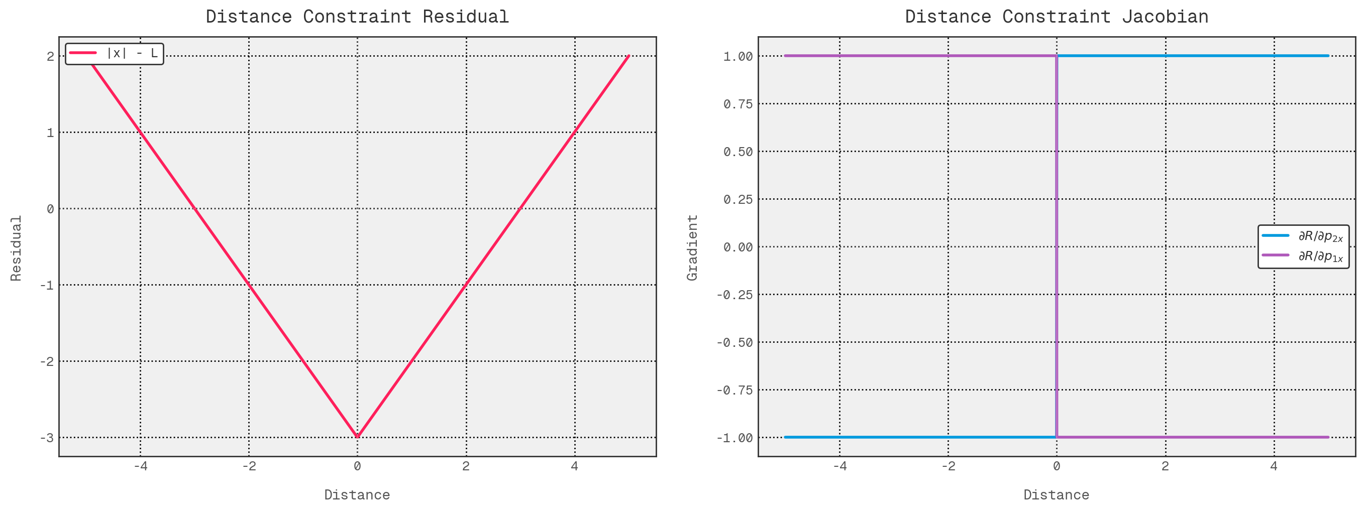
The left hand plot shows the naive residual associated with our distance constraint for a target distance of 3 units:
$$r_{naive}(x) = |x| - L$$Then, on the right hand plot, we have the derivative of that expression:
$$ \frac{dr_{naive}}{dx} = \begin{cases} -1 & x<0\\\\ 1 & x>0 \end{cases} \qquad \text{undefined at }x=0 $$In both the symbols and the plots, the residual is continuous everywhere, but it is not differentiable at $x=0$, where the gradient is undefined. Equivalently, its derivative is $\operatorname{sign}(x)$ for $x \neq 0$, but jumps instantaneously from $-1$ to $+1$ as we pass through the apex of the V. That lack of smoothness is problematic for Newton-type methods, because each iteration assumes a locally smooth function and chooses a step direction from the current linearisation (the Jacobian). Near the turning point, small perturbations can flip the predicted direction, making the step choice unstable and potentially leading to oscillation or slower convergence.
In 1D, the derivative away from zero can only take the values $-1$ or $1$. In 3D, the same idea generalises to a unit vector pointing in the direction of $\vec{d}$:
$$ \frac{\partial r}{\partial \vec{d}} = \begin{cases} \dfrac{\vec{d}}{\lVert \vec{d} \rVert} & \vec{d} \neq \vec{0} \\ \qquad \text{undefined} & \vec{d} = \vec{0} \end{cases} $$Similar to the 1D case, this gradient is well-defined for $\vec{d} \neq \vec{0}$, but undefined at $\vec{d} = \vec{0}$. Near coincident points, its magnitude remains bounded, but its direction becomes extremely sensitive to small perturbations in $\vec{d}$; there is no unique limiting direction as $\vec{d} \to \vec{0}$. That is the 3D analogue of the non-smooth behaviour in the 1D case, and it is similarly awkward for Newton-type methods, which assume locally smooth residuals and Jacobians. Even though the target for a distance constraint is $\lVert \vec{d} \rVert = L$ (not zero unless $L=0$), iterates can still pass near this region during a solve.
So, with EPS_SQ, what we have in there is really a regularised Euclidean norm which we’ve softened in order to remove
that singularity and make the gradient smooth everywhere. To that end, we assemble what I have referred to as a
softnorm:
def softnorm(sum_of_squares: float) -> float:
    """
    Bias-corrected regularised norm: `sqrt(s + EPS_SQ) - EPS`.

    Returns exactly zero when sum_of_squares is zero, with finite derivatives
    everywhere.
    """
    return math.sqrt(sum_of_squares + EPS_SQ) - EPS
Applied to the 3D residual, this gives:
$$ r_{soft}(\vec{d}) = \sqrt{\lVert \vec{d} \rVert^2 + \epsilon^2} - \epsilon - L $$With gradient
$$ \frac{\partial r_{soft}}{\partial \vec{d}} = \dfrac{\vec{d}}{\sqrt{\lVert \vec{d} \rVert^2 + \epsilon^2}} $$This has two nice properties:
- When $\vec{d} = \vec{0}$, the softened norm term evaluates to $\sqrt{\epsilon^2} - \epsilon = 0$, so we remove the singularity without introducing an offset at zero.
- The gradient is finite everywhere. At $\vec{d} = \vec{0}$, it evaluates to $\vec{0}$, which is perfectly well-behaved.
In terms of the actual point coordinates, the partials are then:
$$ \frac{\partial r_{soft}}{\partial {p}_1} = -\dfrac{\vec{d}}{\sqrt{\lVert \vec{d} \rVert^2 + \epsilon^2}} $$And:
$$ \frac{\partial r_{soft}}{\partial {p}_2} = \dfrac{\vec{d}}{\sqrt{\lVert \vec{d} \rVert^2 + \epsilon^2}} $$The $-\epsilon$ term is just a constant bias correction, so it disappears under differentiation; this is why the SymPy-generated Jacobians only contain the $\sqrt{\lVert \vec{d} \rVert^2 + \epsilon^2}$ term.
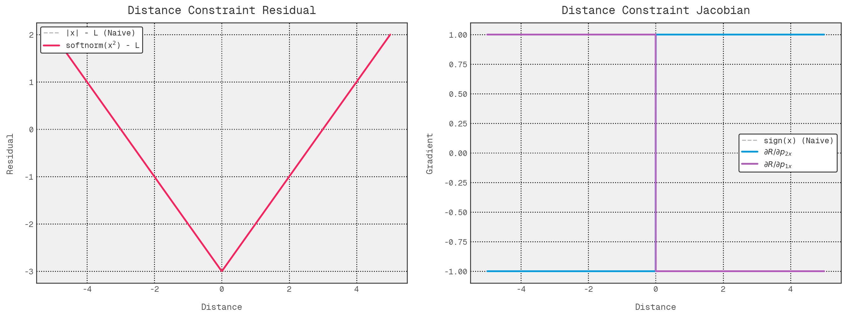
So, going back to our simplified plots, this looks much like before, provided we use a zoomed out view. This shows that, at least at a macro level, our modified residual and gradient functions look exactly like our naive versions, which is exactly what we want.
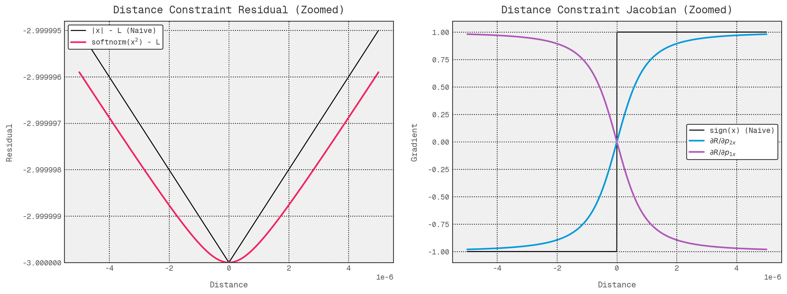
However, zoom in a bit so we can see $\epsilon$ scale changes, and we can see the effect much more clearly. The residual has no abrupt, discontinuous change, and the gradient values blend through the sign change region.
One caveat: our current Jacobian tests validate the analytical derivatives against central differences of the
unregularised residuals (raw norms and cross products), not the softened softnorm versions the solver actually uses.
Away from singularities the two agree closely enough that the tests pass, but we’re not yet verifying the exact softened
Jacobian behaviour near the degeneracies that the regularisation is specifically designed to handle.
We could also look into using squared error terms instead of softnorms here and avoid this work entirely, but then we might get into scaling issues which I’d rather avoid. This might resurface at some point down the road, but for now, we’re running with the softnorm approach.
DIY autodiff, part 1: why?
The approach described above works incredibly well when you have a limited set of fixed derivative expressions which you will use over and over and over again; it becomes worth the up-front effort of computing the true derivatives. However, where the functions whose derivatives you need are highly varied, even arbitrary, then it ceases to be a practical solution.
In the case of our suspension kinematics tool, there’s a slightly unexpected scenario we don’t have restricted functions we can differentiate with SymPy up front: derived points.
Deriving the derivatives of derived points
We set out to design this program such that we can apply sweep targets to derived points, not just the points which actually control the suspension’s motion. To enable this, our objective function, i.e., the vector of residuals we’re trying to minimise, can involve targets set on derived points.
However, as free points are the only things the solver can actually play tunes with, the solver needs to know how changes in the free points affect the derived points. For example, if we want to drive a sweep by moving the wheel center +10mm in Z, the solver needs to know the sensitivity of that wheel centre position to changes in the positions of the ball joints and track rod ends.
For free points, that response is trivial: moving an outer ball joint up by 10 mm simply makes that ball joint 10 mm higher. Derived points, however, are computed from those free variables through a chain of nonlinear geometric functions. Because these points are ‘downstream’ of the actual solver variables, we need a way to propagate gradients through that geometry to get the analytically exact derivatives the Jacobian requires.
We could, I guess, hand-derive these Jacobians with SymPy, but derived point calculations are volatile. They are bespoke constructions of ball joints, offsets, and reference planes that change whenever you tweak the suspension’s logic. Rather than re-grinding symbolic maths for every geometric experiment, we want a way to get exact derivatives through our derived point code without having to think about it.
This is where automatic differentiation comes in, and for us, the key idea is the ‘dual number’.
DIY autodiff, part 2: stuffing derivatives into numbers
A dual number extends a real number with an infinitesimal component, much like how a complex number extends a real with an imaginary component:
$$ \tilde{x} = a + b\varepsilon \qquad \text{where} \qquad \varepsilon \neq 0, \text{ and } \varepsilon^2 = 0 $$Here, $\varepsilon$ is not an imaginary unit like $i$; it is a ‘nilpotent’ element adjoined to the reals, which means it is nonzero but squares to zero. Using this extension as a carrier for derivative information, we can push the dual numbers through whatever computations we like, and the $\varepsilon$ component carries the derivative. For example:
$$\tilde{x} \cdot \tilde{y} = (a + b\varepsilon)(c + d\varepsilon) = ac + (ad + bc)\varepsilon$$The real part gives the value; the dual part gives the derivative. This extends to all differentiable operations: $\sin$, $\cos$, $\sqrt{}$, etc. by implementing the appropriate chain rule in each operation.
In our case, while we could go shopping for a library here, I was curious to see how hard it would be to hand-roll a
dual number based autodiff
utility. The open-kinematics implementation provides DualScalar and DualVec3 types which override arithmetic
operators and hook into numpy’s __array_function__ protocol, so that existing code using np.dot and np.linalg.norm
works transparently with dual inputs:
class DualScalar:
    __slots__ = ("val", "deriv")

    def __init__(self, val: float, deriv: float = 0.0):
        self.val = float(val)
        self.deriv = float(deriv)

    def __mul__(self, other):
        if isinstance(other, DualScalar):
            return DualScalar(
                self.val * other.val,
                self.val * other.deriv + self.deriv * other.val,
            )
        ...
As a concrete example, suppose we want the derivative of this function at $x=2$:
$$ f(x) = x^2 + 3x $$With dual numbers, we evaluate the function not at $2$, but at:
$$ \tilde{x} = 2 + \varepsilon $$Here, the coefficient of $\varepsilon$ is the ‘seed’. In practice, we usually seed with 1 for the variable we are differentiating with respect to, and 0 elsewhere. A seed of 1 means that the dual part of the result will carry the plain derivative with respect to that input. In the univariate case, any other seed value would give a scaled derivative, which is not generally what we want. In the multivariate case, seeding one variable with 1 and the others with 0 gives the corresponding partial derivative. More general seed vectors produce directional derivatives, which is not what we’re after here.
Substituting $\tilde{x} = 2 + \varepsilon$ into the function gives:
$$ f(\tilde{x}) = (2 + \varepsilon)^2 + 3(2 + \varepsilon) $$Expanding and using $\varepsilon^2 = 0$:
$$ f(\tilde{x}) = 4 + 4\varepsilon + \varepsilon^2 + 6 + 3\varepsilon = 10 + 7\varepsilon $$So, from a single evaluation of $f(\tilde{x})$, we get both:
- The function value, $f(2) = 10$.
- The derivative, $f'(2) = 7$.
The real part gives the value; the dual part gives the derivative with respect to the seeded variable.
Running some actual code:
from kinematics.core.dual import DualScalar


def polynomial(x: DualScalar) -> DualScalar:
    """
    Return f(x) = x^2 + 3x.
    """
    return x * x + 3.0 * x


x = 2.0
eps = 1.0

x_tilde = DualScalar(x, eps)
y = polynomial(x_tilde)

print("Function: f(x) = x^2 + 3x")
print(f"x = {x}")
print(f"x_tilde = {x_tilde}")
print(f"y = {y}")
print(f"y.val = {y.val}")
print(f"y.deriv = {y.deriv}")
Gives us:
Function: f(x) = x^2 + 3x
x = 2.0
x_tilde = DualScalar(val=2.0, deriv=1.0)
y = DualScalar(val=10.0, deriv=7.0)
y.val = 10.0
y.deriv = 7.0
The exact mechanism is what lets us differentiate more complicated geometric constructions without having to do any
manual work. We just lean on the chain rule, but we abstract away the requirement to think about the chain rule or
seeding $\varepsilon$ or anything like that. We write our derived point calculations using dual number types for both
scalar and vector quantities, sticking to the operations our Dual class supports (basic arithmetic, dot products,
norms, indexing, and a few NumPy functions). Then we use a seed_positions utility to handle the seeding for each
free-variable coordinate, and we get exact Jacobian rows without having to hand-apply the chain rule.
Note that the coverage isn’t unlimited; a derived point function that bleeds into unsupported NumPy territory would need the dual number layer to be extended first… but it’s enough for the current set of geometric constructions.
def seed_positions(
    positions: dict[PointID, np.ndarray],
    seed_point: PointID,
    seed_dim: int,
) -> dict[PointID, DualVec3]:
    """
    Create dual-number positions seeded for differentiation.

    Wraps every position as a DualVec3 with zero derivative, except
    seed_point which gets derivative = 1.0 in coordinate seed_dim.
    This sets up forward-mode AD to compute d(output)/d(seed_point[seed_dim]).

    Args:
        positions: Current point positions (PointID -> ndarray).
        seed_point: The point whose coordinate we differentiate w.r.t.
        seed_dim: Which coordinate (0=x, 1=y, 2=z) to seed.

    Returns:
        Dictionary of DualVec3 positions ready for derived-point computation.
    """
    dual_positions: dict[PointID, DualVec3] = {}
    for pid, pos in positions.items():
        if pid == seed_point:
            d = np.zeros(3, dtype=np.float64)
            d[seed_dim] = 1.0
            dual_positions[pid] = DualVec3(pos.copy(), d)
        else:
            dual_positions[pid] = DualVec3(pos.copy())
    return dual_positions
Derivative distribution: assembling the full Jacobian
With per-constraint Jacobian functions ironed out, we still have one more thing to do: assemble all of those partial derivatives into the global Jacobian matrix that our solver needs.
This is where the ResidualComputer class comes in. It owns both the residual assembly and the Jacobian assembly, and,
it does as much work as possible up front. At construction time, it:
- Builds a mapping from each free point ID to its column in the solver variable vector.
- Pre-allocates a Jacobian buffer of the maximum required size.
- Pre-computes a per-constraint ‘plan’ describing:
- Which Jacobian function should be called for that constraint, and,
- Where each three element wide block of partial derivatives should be placed into the global Jacobian row.
That planning step matters because each constraint Jacobian is naturally computed in a local coordinate system: if a distance constraint involves two points, its derivative function returns six numbers; three partials for the first point and three for the second, and these must be placed into the appropriate columns of the global Jacobian. As we saw above, our solver variable vector, which corresponds to the coordinates of our free points, is as follows:
$$ x = \begin{bmatrix} p_{1x} & p_{1y} & p_{1z} & p_{2x} & p_{2y} & p_{2z} & \cdots \end{bmatrix} $$So, for each constraint row, we need a mapping from local derivative slots to global column indices. That is what the distribution list provides.
Conceptually, a plan produced by build_jac_plan looks something like:
compute_fn, distribution = (
    jacobian_function_for_this_constraint,
    [
        (0,  6),   # Copy derivs[0:3] into J[row, 6:9].
        (3, 15),   # Copy derivs[3:6] into J[row, 15:18].
    ],
)
The first tuple element in each pair is the offset into the local derivative array returned by the constraint Jacobian function. The second is the starting column in the full Jacobian. Fixed points are simply omitted from this mapping, because they are not solver variables and therefore contribute no columns to the Jacobian.
At solve time, compute_jacobian follows a very simple pattern.
First, just like the residual computation, it updates the working state from the current free variable vector and recomputes any derived points. Because the residual computer is initialised with a fixed target count, the Jacobian has a fixed shape for the lifetime of the solve: one row per geometric constraint plus one row per target variable. So at evaluation time, it simply reuses the full pre-allocated buffer and zeroes it with:
jac[:] = 0.0
For the constraint rows, it loops over the pre-computed plans. Each plan gives it a function to call and a distribution list to apply. The Jacobian function returns the local derivative array for that constraint, and the distribution list tells us exactly where each element of that derivative vector belongs in the global row. Since the plans were built once up front, the solve time loop does not need to re-discover which points are involved in which constraint, or which of those points are free.
Basically, the solve time work for an analytical constraint row is:
derivs = compute_fn(positions)
for d_start, j_col in distribution:
    jac[row, j_col:j_col + 3] = derivs[d_start:d_start + 3]
That’s the whole assembly step: compute local derivatives, then distribute the non-zero blocks into the right places.
Target rows are handled slightly differently. A target residual is always the projection of the point onto the target direction, minus the desired value:
$$ r_{target} = \operatorname{dot}(p, {u}) - \text{value} $$Where $p$ is the point position and ${u}$ is the unit vector for the target direction (e.g. the global $z$-axis for a vertical height target). If the target point is itself a free point, the derivative is trivial: projecting onto a fixed direction is linear, so the Jacobian row is just the direction vector ${u}$ written into the columns for that point.
Derived point targets are more complicated. A point like the wheel centre is not a direct solver variable; as we saw above, it is a nonlinear function of the free points. In that case, we still need a Jacobian row with respect to the free coordinates, but now we have to apply the chain rule through the derived point computation. This is where the dual number machinery from the previous section is applied.
For each free point and each coordinate direction, we create a dual number version of the position dictionary with that one coordinate seeded to 1. We then run the normal derived point update code on those dual positions. The dual part of the resulting target point tells us the sensitivity of that derived point to the seeded input coordinate. Projecting that sensitivity onto the target direction gives the corresponding Jacobian entry:
$$\frac{\partial}{\partial q}\left(\operatorname{dot}(p_{derived}, {u})\right) = \operatorname{dot}\left({u}, \frac{\partial p_{derived}}{\partial q}\right)$$Where $q$ is one coordinate of one free point.
So, for derived point targets, we effectively build the row one scalar entry at a time by seeding each free coordinate in turn, propagating that seed through the derived point computation, and reading out the projected derivative.
The result of all this is a Jacobian assembly scheme with a useful split of responsibilities:
- Fixed, known geometric constraints use pre-generated analytical Jacobian functions plus cheap distribution steps.
- Arbitrary, user-defined derived point constructions use forward-mode autodiff to recover exact sensitivities.
Because the buffer shape and distribution plans are pre-computed, the solve time work stays relatively straightforward; it’s something like:
- Validate the fixed target count,
- Zero the buffer,
- Update the current state,
- Evaluate local derivatives,
- Distribute local derivatives into global Jacobian,
- Fill the target rows,
- Return a copy of the filled matrix.
That gives SciPy a Jacobian which is analytically exact, sparse in structure, and assembled with reduced allocation in the fixed constraint path (buffer shapes and distribution plans are pre-computed, though SciPy’s interface does require a fresh copy of the filled matrix each call).
Metrics
As interesting as the above is, our overarching objective with all this is to assemble a tool which can help us understand and improve the behaviour of our suspension systems. To that end, we need plots. Plots help us to get information about the system into our brains, and that helps us make better decisions about what to do next.
At present, we only simulate one corner at a time, so some metrics are out of reach for now (ride height, roll centre height, and anything else that depends on a better estimation of vehicle attitude). But there are still a bunch of useful values which we can compute. By my reckoning, we can get:
- Wheel centre position.
- Camber angle.
- Caster angle.
- Roadwheel angle.
- KPI.
- Scrub radius.
- Mechanical trail.
In general, things are quoted in chassis-relative values, so it may be more useful to talk about the change in these values relative to the static configuration, rather than their absolute values. For example, we might be more interested in the change in camber angle as the suspension compresses, rather than the true inclination of the wheel centre plane relative to some notion of ground.
On ground planes
At the moment, I’m not entirely convinced of the best way to handle ground plane references. I haven’t spent a great deal of time thinking about it, and it’s been 7 or 8 years since I used a tool like this written by someone else… so I can’t remember how other products deal with it. I could maybe persuade myself that you can get away with a fixed chassis model and working almost entirely with deltas relative to the static condition… but I’m not sure. For example, I could imagine a simulation sweep being supplied alongside design condition values for ride height, then computing and applying offsets.
However, that’s not what we do at present. With the current setup, any metrics which require some ground plane reference use a simple model: we imagine an infinitely thin disc lying in the wheel centre plane, and the lowest point on that disc we consider to be our contact patch centre. The horizontal plane through that point, parallel to the world XY plane, is our ground plane. I suspect this isn’t too bad an approach; we should be able to extend it to a full axle model, and I always find it easier to reason about things in absolute units rather than deltas on deltas on deltas.
Practically, to find that low point on the wheel centre plane disc, we start from the centroid and move in the wheel centre plane ‘down’ direction by the nominal tyre radius. That wheel centre plane down vector is the component of global down, i.e., $-Z$, which lies in the wheel centre plane. This is effectively global down with any component parallel to the axle axis removed. So if ${a}_{wheel}$ is the axle direction and ${z}$ is global up, then:
$$ v_{wheelDown} = \operatorname{normalize}\left( -{z} - \left((-{z}) \cdot {a}_{wheel}\right){a}_{wheel} \right) $$Therefore:
$$ p_{contactPatch} = p_{wheelCenter} + r_{tyre}v_{wheelDown} $$The $Z$ coordinate of this contact patch point is what we treat as ground level. Any metric which needs a ground plane intersection (scrub radius, mechanical trail etc.) uses the horizontal plane at $p_{contactPatchZ}$.
For those metrics, we also need the point where the steering axis meets that plane. Parameterising the steering axis as a line through the lower and upper balljoints:
$$ p_{steering}(t) = p_{lowerBalljoint} + t\left(p_{upperBalljoint} - p_{lowerBalljoint}\right) $$We solve for the value of $t$ which gives the same $Z$ coordinate as the contact patch centre:
$$ t_{ground} = \frac{p_{contactPatchZ} - p_{lowerBalljointZ}} {p_{upperBalljointZ} - p_{lowerBalljointZ}} $$Which gives:
$$ p_{ground} = p_{steering}(t_{ground}) $$In code, that is what our MetricContext.steering_axis_ground_intersection is doing.
    def steering_axis_ground_intersection(self) -> Vec3 | None:
        """
        Point where the steering axis intersects the ground plane.

        Parameterises the line from the lower ball joint through the upper
        ball joint and solves for the parameter t where Z = ground_z.
        Returns None if the steering axis is parallel to the ground plane.
        """
        lower = self.state.get(PointID.LOWER_WISHBONE_OUTBOARD)
        upper = self.state.get(PointID.UPPER_WISHBONE_OUTBOARD)
        direction = upper - lower
        dz = direction[Axis.Z]
        if abs(dz) < EPS_GEOMETRIC:
            return None
        # t such that lower + t * direction has Z = ground_z
        t = (self.ground_z - lower[Axis.Z]) / dz
        return lower + t * direction
We can try this for now; it should give us internally consistent values for ‘contact patch’ location, scrub radius, and mechanical trail in the context of the disc tangent model. Though it’s worth noting that these values are tied to this specific ground plane approximation; a different ground model. A better approach to ground plane estimation is probably worth investigating at some point.
Camber, caster, toe
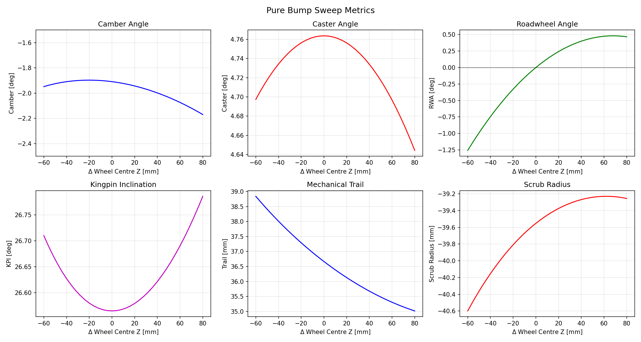
Camber and toe/roadwheel angle (or their rate of change wrt. vertical hub displacement) are likely to be two of the most well-known metrics here, so let’s start with these. Note that the plots below show absolute angles rather than deltas from the static condition; what you’re seeing is total camber and roadwheel angle across the sweep, not camber gain or bump steer as commonly understood.
The nice thing about these three is that, once we have a solved suspension state, they reduce to straightforward vector
geometry. In open-kinematics, we build a small per-state metrics context and cache a couple of shared geometric
quantities:
- The wheel axis, taken as the unit vector from axle inboard to axle outboard.
- The steering axis, taken as the unit vector from lower balljoint to upper balljoint.
Using the ISO 8855 convention, that means $X$ is forward, $Y$ is left, and $Z$ is up.
For camber and toe, the starting point is the wheel axis:
$$ {a}_{wheel} = \operatorname{normalize}\left( p_{axleOutboard} - p_{axleInboard} \right) $$For caster, the starting point is the steering axis:
$$ {a}_{steering} = \operatorname{normalize}\left( p_{upperBalljoint} - p_{lowerBalljoint} \right) $$From there, each metric is just a projection into the plane we care about, followed by an atan2.
Camber
Camber is measured in the front view, so we want the inclination of the wheel relative to the global vertical axis in the $YZ$ plane. So we need the direction in which the wheel centre plane intersects the front view ($YZ$) plane; we can get that by taking the cross product of the wheel axis with the vehicle $X$ axis:
$$ v_{wheelUp} = {a}_{wheel} \times {x} $$Because left and right corners have opposite handedness, we then flip this vector according to vehicle side so that it consistently points upward:
$$ v_{wheelUp}^{*} = -s \left( {a}_{wheel} \times {x} \right) $$Where $s = 1$ for the left-hand side and $s = -1$ for the right-hand side.
Now we can just look at the $Y$ and $Z$ components of that vector and measure its angle relative to vertical:
$$ \theta_{camberRaw} = \operatorname{atan2}\left(v_{wheelUpY}^{*}, v_{wheelUpZ}^{*}\right) $$To keep the sign convention intuitive, we then apply one final side-dependent sign correction. The end result is that negative camber means the top of the wheel is tilted inward toward the vehicle centreline on either side of the car.
Caster
Caster is a bit more straightforward. Here we look directly at the steering axis in side view, so we project ${a}_{steering}$ into the $XZ$ plane and measure its angle relative to the global $Z$ axis:
$$ \theta_{caster} = \operatorname{atan2}\left(-{a}_{steeringX}, {a}_{steeringZ}\right) $$The minus sign on the $X$ component is just a convention. It ensures that positive caster corresponds to the top of the steering axis being tilted rearward relative to the lower balljoint. So if the upper balljoint sits behind the lower balljoint, caster comes out positive.
Toe
For toe, we go back to the wheel axis and look at it in plan view. Projecting the wheel axis into the $XY$ plane gives us the orientation of the wheel around the vertical axis. For the left hand side, we get:
$$ \theta_{toe,left} = \operatorname{atan2}\left({a}_{wheelX}, {a}_{wheelY}\right) $$And for the right hand side:
$$ \theta_{toe,right} = \operatorname{atan2}\left({a}_{wheelX}, -{a}_{wheelY}\right) $$Again, the side-dependent handling is purely there to make the sign convention line up with how we actually talk about the car. Positive toe means toe-in: the front of the wheel points toward the vehicle centreline. Negative toe means toe-out.
The implementation exports this quantity as roadwheel_angle_deg, and we generally refer to roadwheel angle rather than
toe, largely in the interest of clarity.
So, in implementation terms, these three metrics are all the same pattern:
- Build the physically meaningful axis from solved point positions.
- Project that axis, or a derived axis, into the relevant view plane.
- Use
atan2so the sign behaves correctly through all quadrants. - Apply whatever side specific sign handling is needed so left and right corners follow the same engineering convention.
That is enough to give us corner-level camber, caster, and toe traces directly from the solved geometry.
KPI, scrub radius, and mechanical trail
The other values we can compute readily at this point are KPI, scrub radius, and mechanical trail. These all describe the position and orientation of the steering axis relative to the wheel and ground, using the same steering axis ${a}_{steering}$ and the contact patch and ground intersection points established above.
For KPI, only the steering axis direction is needed. For scrub radius and mechanical trail, we use the two reference points from our ground model: $p_{contactPatch}$ and $p_{ground}$. Scrub radius and trail are then just signed distances between those points in front and side view respectively.
KPI
KPI is the front-view inclination of the steering axis, measured relative to the global vertical axis in the $YZ$ plane. It is therefore the direct counterpart to caster, just in the other view:
$$ \theta_{KPI} = \operatorname{atan2}\left(-s \cdot {a}_{steeringY}, {a}_{steeringZ}\right) $$Where again $s = 1$ on the left-hand side and $s = -1$ on the right-hand side.
That side specific sign handling ensures that positive KPI means the top of the steering axis is tilted inward toward the vehicle centreline on either side of the car. In other words, positive KPI means the upper balljoint is more inboard than the lower balljoint.
Scrub radius
Scrub radius is the lateral distance, measured in the ground plane, between the contact patch centre and the point where the steering axis intersects the ground.
We take scrub radius as positive when the steering axis meets the ground inboard of the contact patch, and negative when it meets the ground outboard.
In implementation terms, we project the displacement from the contact patch to the steering axis ground intersection onto the wheel’s lateral direction in the ground plane. To get that lateral direction, we take the wheel axle axis ${a}_{wheel}$, zero its vertical component, and re-normalise:
$$ {a}_{wheelGround} = \operatorname{normalize}\left( \begin{bmatrix} {a}_{wheelX} \\ {a}_{wheelY} \\ 0 \end{bmatrix} \right) $$$$ r_{scrub} = -\operatorname{dot}\left(p_{ground} - p_{contactPatch},\; {a}_{wheelGround}\right) $$Because ${a}_{wheelGround}$ already points outboard on each side of the car, the same expression works on both left and right corners without an explicit side factor.
Mechanical trail
Mechanical trail is the longitudinal distance between the steering axis reference-plane intersection and the contact patch centre:
$$ t_{mechanical} = p_{groundX} - p_{contactPatchX} $$Using ISO 8855, positive $X$ is forward, so positive mechanical trail means the contact patch sits behind the steering axis reference-plane intersection. That is the usual self-centring case: the tyre force acts at a point trailing behind the axis about which the wheel steers.
Unlike scrub radius and KPI, no left-right sign adjustment is needed here because fore-aft direction is shared by both sides of the car.
Taken together, these three values give a pretty good first-order description of where the steering axis lives in space relative to the tyre. KPI tells us how much that axis leans inward in front view, scrub radius tells us where it lands laterally at ground level, and mechanical trail tells us where it lands longitudinally.
The plots
Once we put all that together and run a bump sweep, we can finally start pulling together useful results sets for realistic suspensions. For our example suspension with a pure bump sweep like this:
We would be able to produce a set of metrics like this:
Further work
The tool is now in a fairly good place; with a little bit of validation, I think you could almost use it to do some actual work on a real car. However, there are still a few things missing which would make it quite a bit more powerful.
By my reckoning, we need:
- A full axle model, with some mechanism for specifying sweeps to include roll displacement.
- A better ground plane model. The current disc tangent approach (described above) is a reasonable starting point, but some metrics we want depend on ground plane reference. A fixed road plane derived from a vehicle attitude calc might be more representative, and would also let us compute ride height and roll centre height under different conditions.
- Some validation against another tool. A CAD system with some kinematics or assembly constraint capabilities, or a dedicated suspension analysis tool, or perhaps a setup using something like MIT’s Drake.
- Better visualisation of results, though this may be better tackled through a separate app.
- At a push, some outer solver loop which would allow us to specify the desired characteristics of the system, and then have the program automatically tweak the geometry to try to achieve those targets.